SARSA in the Wind
We will use SARSA algorithm to find the optimal policy so that our agent can navigate in windy world.
SARSA
State–action–reward–state–action (SARSA) is an algorithm for learning a Markov decision process policy, used in the reinforcement learning area of machine learning.
SARSA focuses on state-action values.
It updates the Q-function based on the following equation:
Q(s,a) = Q(s,a) + α (r + γ Q(s’,a’) – Q(s,a))
Here s’ is the resulting state after taking tha action ,a, in state s;
r is the associated reward;
α is the learning rate
and γ is the discount factor.
Windy GridWorld
Windy Gridworld is a grid problem with a 7 * 10 board, which is displayed as follows:
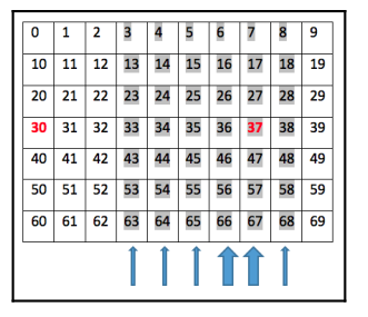
An agent makes a move up, right, down, and left at a step. Tile 30 is the starting point for
the agent, and tile 37 is the winning point where an episode will end if it is reached. Each
step the agent takes incurs a -1 reward.
The complexity in this environment is that there is extra wind force in columns 4 to 9.
Moving from tiles on those columns, the agent will experience an extra push upward. The
wind force in the seventh and eighth columns is 1, and the wind force in the fourth, fifth,
sixth, and ninth columns is 2. For example, if the agent tries to move right from state 43,
they will land in state 34; if the agent tries to move left from state 48, they will land in state
37; if the agent tries to move up from state 67, they will land in state 37 as the agent receives
an additional 2-unit force upward; if the agent tries to move down from state 27, they will
land in state 17, as the 2 extra force upward offsets 1 downward.
Developing the Windy Gridworld environment:
#Import the basic libraries
import numpy as np
import sys
from gym.envs.toy_text import discrete
#Define actions
UP = 0
RIGHT = 1
DOWN = 2
LEFT = 3#The gridworld calss
class WindyGridworldEnv(discrete.DiscreteEnv):
def __init__(self):
self.shape = (7,10)
nS = self.shape[0]*self.shape[1]
nA = 4
#Winds locations
winds = np.zeros(self.shape)
winds[:,[3,4,5,8]]=1
winds[:,[6,7]]=2
self.goal = (3,7)
#Calcualte transition probabiliites and rewards
P = {}
for s in range(nS):
position = np.unravel_index(s,self.shape)
#print(position)
P[s] = {a:[] for a in range(nA)}
P[s][UP] = self._calculate_transition_prob(position,
[-1,0],winds)
P[s][RIGHT] = self._calculate_transition_prob(position,
[0,1],winds)
P[s][DOWN] = self._calculate_transition_prob(position,[1,0],
winds)
P[s][LEFT] = self._calculate_transition_prob(position,[0,-1],winds)
#print(P)
#Calculate initial state distribution
#We start in state (3,0)
isd = np.zeros(nS)
isd[np.ravel_multi_index((3,0),self.shape)] = 1.0
super(WindyGridworldEnv,self).__init__(nS,nA,P,isd)
def _calculate_transition_prob(self,current,delta,winds):
"""
Determine the outcome for an action.
Transition Prob is always 1.0
@param current: (row,col), current position on the grid
@param delta: Changein position for transition
@param winds: Wind effect
@return: (1.0,new_state,reward,is_done)
"""
new_position = np.array(current) + np.array(delta) + np.array([-1,0])*winds[tuple(current)]
new_position = self._limit_coordinates(new_position).astype(int)
new_state = np.ravel_multi_index(tuple(new_position),self.shape)
is_done = tuple(new_position) == self.goal
return [(1.0,new_state,-1.0,is_done)]
def _limit_coordinates(self,coord):
coord[0] = min(coord[0],self.shape[0] -1)
coord[0] = max(coord[0],0)
coord[1] = min(coord[1],self.shape[1]-1)
coord[1] = max(coord[1],0)
return coord
def render(self):
# x represents the agent's current position.
# T is the foal tile
# the remaining tiles are denoted as o
outfile = sys.stdout
for s in range(self.nS):
position = np.unravel_index(s,self.shape)
if self.s == s:
output = 'x'
elif position == self.goal:
output = "T"
else:
output = "o"
if position[1] == 0:
output = output.lstrip()
if position[1] == self.shape[1]-1:
output = output.rstrip()
output += "\n"
outfile.write(output)
outfile.write("\n")
Instantiate an object of Windy Gridworld and playing with it
env = WindyGridworldEnv()env.reset()
env.render()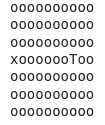
print(env.step(UP))
env.render()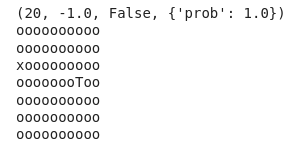
env.s = 43
env.render()
env.step(RIGHT)
env.render()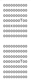
env.s = 48
env.render()
env.step(LEFT)
env.render()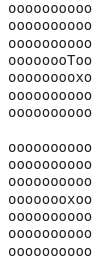
env.s = 47
env.render()
env.step(LEFT)
env.render()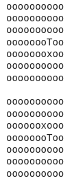
The SARSA Function
import torchdef gen_epsilon_greedy_policy(n_action,epsilon):
def policy_function(state,Q):
probs = torch.ones(n_action)*epsilon/n_action
best_action = torch.argmax(Q[state]).item()
probs[best_action] += 1.0 - epsilon
action = torch.multinomial(probs,1).item()
return action
return policy_functionn_episode = 500
length_episode = [0]*n_episode
total_reward_episode = [0]*n_episodefrom collections import defaultdict
def sarsa(env,gamma,n_episode,alpha):
"""
Obtaion the optimal policy with on-policy SARSA algorithm
@param env: OpenAI Gym environment
@param gamma: discount factor
@param n_episode: number of episodes
@return : The optimal Q-function and the optimal policy
"""
n_action = env.action_space.n
Q = defaultdict(lambda: torch.zeros(n_action))
for episode in range(n_episode):
state = env.reset()
is_done = False
action = epsilon_greedy_policy(state,Q)
while not is_done:
next_state,reward, is_done, info = env.step(action)
next_action = epsilon_greedy_policy(next_state,Q)
td_delta = reward + gamma * Q[next_state][next_action] - Q[state][action]
Q[state][action] += alpha * td_delta
length_episode[episode] += 1
total_reward_episode[episode] += reward
if is_done:
break
state = next_state
action = next_action
policy = {}
for state,actions in Q.items():
policy[state] = torch.argmax(actions).item()
return Q,policy Finding The Optimal Policy with SARSA
#The hyperparameters
gamma = 1
alpha = 0.4
epsilon = 0.1
epsilon_greedy_policy = gen_epsilon_greedy_policy(env.action_space.n,epsilon)optimal_Q, optimal_policy = sarsa(env,gamma,n_episode,alpha)print('The optimal policy: \n',optimal_policy)The optimal policy: {30: 1, 20: 1, 10: 2, 21: 1, 11: 1, 12: 1, 2: 0, 3: 1, 4: 1, 5: 1, 6: 1, 7: 1, 8: 1, 9: 2, 19: 2, 29: 2, 18: 2, 13: 1, 1: 1, 22: 1, 23: 1, 0: 2, 39: 2, 28: 2, 32: 1, 31: 1, 33: 1, 40: 2, 14: 1, 41: 1, 42: 1, 43: 1, 38: 2, 50: 2, 51: 1, 52: 1, 53: 3, 24: 1, 34: 1, 61: 1, 62: 1, 44: 1, 15: 1, 17: 0, 49: 2, 59: 3, 48: 3, 69: 3, 68: 2, 27: 0, 60: 1, 63: 1, 25: 1, 37: 0, 54: 1, 45: 1, 16: 2, 35: 1, 58: 3, 47: 2, 57: 2, 36: 2, 26: 2}
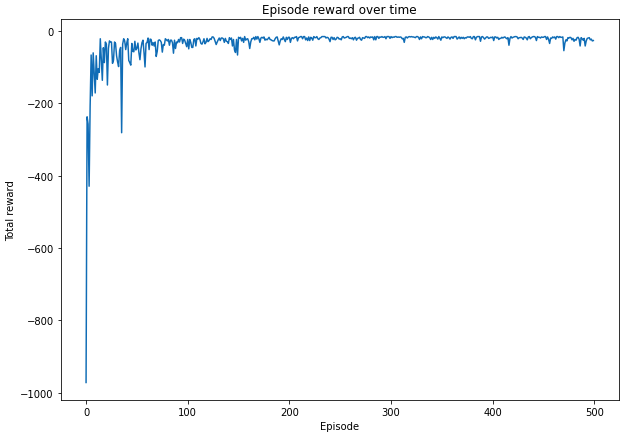
Plotting Episode Length and Reward
import matplotlib.pyplot as plt
plt.figure(figsize=(10,7))
plt.plot(length_episode)
plt.title('Episode length over time')
plt.xlabel('Episode')
plt.ylabel('Length')
plt.show()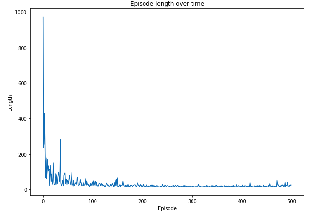
plt.figure(figsize=(10,7))
plt.plot(total_reward_episode)
plt.title('Episode reward over time')
plt.xlabel('Episode')
plt.ylabel('Total reward')
plt.show()