LSTM in PyTorch
Basic of LSTM using PyTorch
Basic import
import torch
import numpy as np
import torch
import torch.nn as nn
Seeding
#Manual seed
torch.manual_seed(786)
Input to feed LSTM network
#random data of 1x6
input = torch.rand(1,6)
print('The size of input: ',input.size())
print('The input itself: ',input)
The size of input: torch.Size([1, 6])
The input itself: tensor([[0.7105, 0.8111, 0.7059, 0.6854, 0.8432, 0.6766]])
Minimal LSTM in PyTorch
#input_size – The number of expected features in the input x
#hidden_size – The number of features in the hidden state h
#nn.LSTM(input_size,hidden_size)
conv,a = nn.LSTM(6,6)(input)
print("The output of above LSTM model:\n ",conv)
print("The value of hidden states:\n ",a)
The output of above LSTM model:
tensor([[ 0.1748, -0.0426, -0.0335, 0.1421, -0.1876, 0.1138]],
grad_fn=<SqueezeBackward1>)
The value of hidden states:
(tensor([[ 0.1748, -0.0426, -0.0335, 0.1421, -0.1876, 0.1138]],
grad_fn=<SqueezeBackward1>), tensor([[ 0.3817, -0.1098, -0.0467, 0.3663, -0.3186, 0.1684]],
grad_fn=<SqueezeBackward1>))
By default the no_of_layer (no of stacked LSTM layers is one)
Let us change it to two
conv,a = nn.LSTM(6,6,2)(input)
print("The output of above LSTM model:\n ",conv)
print('\n')
print("The value of hidden states:\n ",a)
The output of above LSTM model:
tensor([[-0.0099, 0.1247, -0.0815, -0.0407, -0.0446, -0.0919]],
grad_fn=<SqueezeBackward1>)
The value of hidden states:
(tensor([[-0.1088, -0.0990, -0.1030, -0.0013, 0.0947, -0.2360],
[-0.0099, 0.1247, -0.0815, -0.0407, -0.0446, -0.0919]],
grad_fn=<SqueezeBackward1>), tensor([[-0.2402, -0.1555, -0.1816, -0.0034, 0.2623, -0.4411],
[-0.0226, 0.2425, -0.2008, -0.0656, -0.1035, -0.2683]],
grad_fn=<SqueezeBackward1>))Adding Dropout
If non-zero, introduces a Dropout layer on the outputs of each LSTM layer except the last layer,
with dropout probability equal to dropout. Default: 0
conv,a = nn.LSTM(6,6,2,dropout=0.2)(input)
print("The output of above LSTM model:\n ",conv)
print('\n')
print("The value of hidden states:\n ",a)
The output of above LSTM model: tensor([[ 0.2041, 0.0515, -0.0755, 0.1436, -0.0792, 0.0479]], grad_fn=<SqueezeBackward1>)
The value of hidden states: (tensor([[ 0.0369, 0.0682, -0.0806, -0.0235, 0.2393, -0.0630], [ 0.2041, 0.0515, -0.0755, 0.1436, -0.0792, 0.0479]], grad_fn=<SqueezeBackward1>), tensor([[ 0.0664, 0.1654, -0.1296, -0.0542, 0.4706, -0.1871], [ 0.3184, 0.1032, -0.1605, 0.2295, -0.1394, 0.0994]], grad_fn=<SqueezeBackward1>))
Removing bias in LSTM network
conv,a = nn.LSTM(6,6,2,bias=False)(input)
print("The output of above LSTM model:\n ",conv)
print('\n')
print("The value of hidden states:\n ",a)
The output of above LSTM model: tensor([[ 0.0011, -0.0173, 0.0305, -0.0188, -0.0076, -0.0128]], grad_fn=<SqueezeBackward1>)
The value of hidden states: (tensor([[-0.0957, 0.1377, 0.1175, -0.0795, -0.1117, -0.1325], [ 0.0011, -0.0173, 0.0305, -0.0188, -0.0076, -0.0128]], grad_fn=<SqueezeBackward1>), tensor([[-0.1543, 0.2412, 0.2237, -0.1845, -0.2104, -0.3758], [ 0.0023, -0.0348, 0.0591, -0.0390, -0.0159, -0.0243]], grad_fn=<SqueezeBackward1>))
proj_size If > 0, will use LSTM with projections of corresponding size. Default: 0
conv,a = nn.LSTM(6,6,2,proj_size=1)(input)
print("The output of above LSTM model:\n ",conv)
The output of above LSTM model: tensor([[-0.0351]], grad_fn=<SqueezeBackward1>)
conv,a = nn.LSTM(6,6,2,proj_size=2)(input)
print("The output of above LSTM model:\n ",conv)
The output of above LSTM model: tensor([[0.0595, 0.0752]], grad_fn=<SqueezeBackward1>)
#This code generates error
conv,a = nn.LSTM(6,6,2,proj_size=9)(input)
print("The output of above LSTM model:\n ",conv)
ValueError: proj_size has to be smaller than hidden_size
Bidirectional LSTM
#For bidirectional LSTM
#set bidirectional = True
conv,a = nn.LSTM(6,6,bidirectional = True)(input)
print("The output of above LSTM model:\n ",conv)
The output of above LSTM model: tensor([[ 0.1565, -0.2395, 0.1214, 0.1388, 0.1355, 0.0832, 0.0119, -0.0008, -0.2532, 0.1530, -0.0492, 0.0215]], grad_fn=<SqueezeBackward1>)
conv,a = nn.LSTM(6,6,bidirectional = True,proj_size=2)(input)
print("The output of above LSTM model:\n ",conv)
The output of above LSTM model: tensor([[ 0.2349, -0.0812, -0.0632, 0.0543]], grad_fn=<SqueezeBackward1>)
Feeding output of LSTM to linear layer
#preparing the input
input = torch.rand(1,6)
print('The size of input: ',input.size())
print('The input itself: ',input)
The size of input: torch.Size([1, 6]) The input itself: tensor([[0.1132, 0.0979, 0.5497, 0.1461, 0.5804, 0.8175]])
#A LSTM layer
#Followed by ReLU activation function
#The output of LSTM is fed to linear layer
#Which is the fed to ReLU
conv,a = nn.LSTM(6,4)(input)
conv = nn.ReLU()(conv)
conv = nn.Linear(4, 3)(conv)
conv = nn.ReLU()(conv)
print('The final output: \n',conv)
print('The size of final output: \n',conv.size())
The final output: tensor([[0.4911, 0.4870, 0.2221]], grad_fn=<ReluBackward0>)
The size of final output: torch.Size([1, 3])
A complete model
#This is just a helper function
# LSTM() returns tuple of (tensor, (recurrent state))
class extract_tensor_3d_input(torch.nn.Module):
    def forward(self,x):
        # Output shape (batch, features, hidden)
        tensor, _ = x
        # Reshape shape (batch, hidden)
        return tensor[:, -1]
model_lstm_linear = torch.nn.Sequential(
torch.nn.LSTM(6,6),
extract_tensor_3d_input(),
torch.nn.ReLU(),
torch.nn.Linear(6, 20),
torch.nn.ReLU(),
torch.nn.Linear(20,20),
torch.nn.ReLU(),
torch.nn.Linear(20, 1),
torch.nn.Sigmoid()
)#Loss function
loss_func = nn.MSELoss()
#setting Stochastic gradient descent as an optimizer
from torch.optim import SGD
opt = SGD(model_lstm_linear.parameters(),lr=0.001)#Preparing the input and output
input_data = torch.rand(50,1,6)
print('The size of input: ',input_data.size())
t = torch.randn(50).uniform_(0,1)
output_data = torch.bernoulli(t)
print("The output data: \n",output_data.size())
x = input_data
y = output_dataThe size of input: torch.Size([50, 1, 6])
The output data: torch.Size([50])
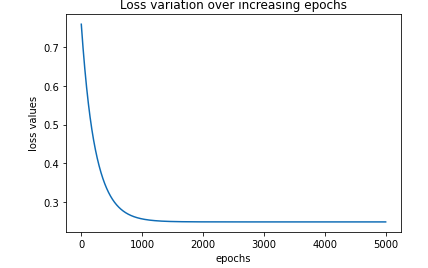
Training the model for 5000 epochs and recording time and loss history
import time
loss_history = []
ticks = time.time()
for _ in range(5000):
  opt.zero_grad()

  loss_value = loss_func(model_lstm_linear(x),y)

  loss_value.backward()
  opt.step()

  loss_value = loss_value.cpu().data.numpy()

  #loss_value = loss_value.numpy()
  loss_history.append(loss_value)
toc = time.time()
print("\n time taken: {}".format(toc-ticks))
time taken: 38.14278554916382
Plotting the loss history
import matplotlib.pyplot as plt
%matplotlib inline

plt.plot(loss_history)
plt.title('Loss variation over increasing epochs')
plt.xlabel('epochs')
plt.ylabel('loss values')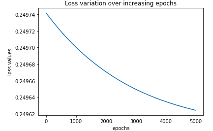
Above model but takes batch of data at a time
model_lstm_linear_batch =  torch.nn.Sequential(
                        torch.nn.LSTM(6,6,batch_first=True),
                        extract_tensor_3d_input(),
                        torch.nn.ReLU(),
                        torch.nn.Linear(6, 20),
                        torch.nn.ReLU(),
                        torch.nn.Linear(20,20),
                        torch.nn.ReLU(),
                        torch.nn.Linear(20, 1),
                        torch.nn.Sigmoid()

                )
#Loss function
loss_func = nn.MSELoss()
#setting Stochastic gradient descent as an optimizer
from torch.optim import SGD
opt = SGD(model_lstm_linear_batch.parameters(),lr=0.001)loss_history = []
ticks = time.time()
for _ in range(5000):
opt.zero_grad()
loss_value = loss_func(model_lstm_linear_batch(x),y)
loss_value.backward()
opt.step()
loss_value = loss_value.cpu().data.numpy()
#loss_value = loss_value.numpy()
loss_history.append(loss_value)
toc = time.time()
print("\n time taken: {}".format(toc-ticks))time taken: 4.788837432861328
%matplotlib inline

plt.plot(loss_history)
plt.title('Loss variation over increasing epochs')
plt.xlabel('epochs')
plt.ylabel('loss values')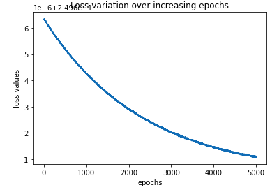
Making models with class
#Class of neural network with LSTM followed by linear layers
class My_LSTM_NeuralNet(nn.Module):
  def __init__(self):
    super().__init__()
    #define LSTM layer
    self.lstm_layer = nn.LSTM(6,6)

    #define hidden layer
    self.input_to_hidden_layer = nn.Linear(6,4)
    #define activation function of hidden layer
    self.hidden_layer_activation = nn.ReLU()
    #define output layer
    self.hidden_to_output_layer = nn.Linear(4,1)

  #Define feed forward network based on above definitions
  def forward(self,x):
        x,_ = self.lstm_layer(x)
        x = self.hidden_layer_activation(x)
        x = self.input_to_hidden_layer(x)
        x = self.hidden_layer_activation(x)
        x = self.hidden_to_output_layer(x)
        return x
my_lstm_net = My_LSTM_NeuralNet()#Loss function
loss_func = nn.MSELoss()
opt = SGD(my_lstm_net.parameters(),lr=0.001)loss_history = []
ticks = time.time()
for _ in range(5000):
opt.zero_grad()
loss_value = loss_func(my_lstm_net(x),y)
loss_value.backward()
opt.step()
loss_value = loss_value.cpu().data.numpy()
#loss_value = loss_value.numpy()
loss_history.append(loss_value)
toc = time.time()
print(toc-ticks)Time taken : 41.547165393829346 seconds
Plotting the loss
%matplotlib inline

plt.plot(loss_history)
plt.title('Loss variation over increasing epochs')
plt.xlabel('epochs')
plt.ylabel('loss values')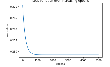
Class of LSTM which takes batch of data
#Class of neural network with LSTM followed by linear layers
class My_LSTM_NeuralNet_batch(nn.Module):
  def __init__(self):
    super().__init__()
    #define LSTM layer
    self.lstm_layer = nn.LSTM(6,6,batch_first=True)

    #define hidden layer
    self.input_to_hidden_layer = nn.Linear(6,4)
    #define activation function of hidden layer
    self.hidden_layer_activation = nn.ReLU()
    #define output layer
    self.hidden_to_output_layer = nn.Linear(4,1)

  #Define feed forward network based on above definitions
  def forward(self,x):
        x,_ = self.lstm_layer(x)
        x = self.hidden_layer_activation(x)
        x = self.input_to_hidden_layer(x)
        x = self.hidden_layer_activation(x)
        x = self.hidden_to_output_layer(x)
        return x
my_lstm_net_batch = My_LSTM_NeuralNet_batch()#Loss function
loss_func = nn.MSELoss()
opt = SGD(my_lstm_net_batch.parameters(),lr=0.001)loss_history = []
ticks = time.time()
for _ in range(5000):
opt.zero_grad()
loss_value = loss_func(my_lstm_net_batch(x),y)
loss_value.backward()
opt.step()
loss_value = loss_value.cpu().data.numpy()
#loss_value = loss_value.numpy()
loss_history.append(loss_value)
toc = time.time()
print("Time taken: ",toc-ticks)Time taken: 4.252270698547363
Plotting the Loss
%matplotlib inline

plt.plot(loss_history)
plt.title('Loss variation over increasing epochs')
plt.xlabel('epochs')
plt.ylabel('loss values')