Python

Logistic Regression in PyTorch
Load the Data
import pandas as pd
import numpy as np
#read csv file
circles = pd.read_csv('.../circles.csv',index_col=0)
circles.head()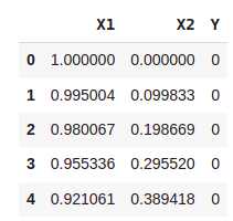
Converting each column data to numpy array
x1 = circles['X1'].values
x2 = circles['X2'].values
y = circles['Y'].values
#combining two inputs in one
x = [x1,x2]
From numpy array to pytorch tensor
import torch
X = torch.Tensor(x)
Y = torch.Tensor(y)
#Transposing input
X = torch.transpose(X,0,1)
Plotting the data
import matplotlib.pyplot as plt
plt.scatter(X[:,0],X[:,1],c=Y)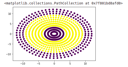
Using the GPU
#preparing output for neural network
Y = torch.unsqueeze(Y,1)
device = 'cuda' if torch.cuda.is_available() else 'cpu'
X = X.to(device)
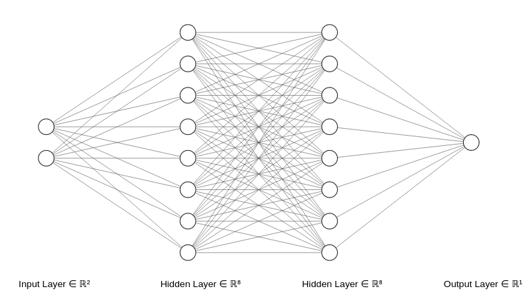
Y = Y.to(device)Defining the neural network
import torch.nn as nnclass MyNeuralNet(nn.Module):
def __init__(self):
super().__init__()
#define hidden layer
self.input_to_hidden_layer = nn.Linear(2,8)
#define activation function of hidden layer
self.hidden_layer_activation = nn.ReLU()
#define hidden layer
self.hidden_layer_to_hidden_layer = nn.Linear(8,8)
#define output layer
self.hidden_to_output_layer = nn.Linear(8,1)
#define activation function of output layer
self.output_layer_activation = nn.Sigmoid()
#Define feed forward network based on above definitions
def forward(self,x):
x = self.input_to_hidden_layer(x)
x = self.hidden_layer_activation(x)
x = self.hidden_layer_to_hidden_layer(x)
x = self.hidden_layer_activation(x)
x = self.hidden_to_output_layer(x)
x = self.output_layer_activation(x)
return x
Putting neural network on GPU
mynet = MyNeuralNet().to(device)Loss function
#Binary cross entropy
loss_func =  torch.nn.BCELoss()
Setting ADAM as an optimizer
from torch.optim import Adam
opt = Adam(mynet.parameters(),lr=0.01)
Defining accuracy
def accuracy(Y,z):
  #returns accuracy and y_hat
  y_hat = torch.round(z.data)
  is_correct = y_hat == Y

  is_correct = is_correct.cpu().numpy().tolist()

  val_epoch_accuracies = np.mean(is_correct)
  Y_hat = y_hat.cpu().data.numpy()

  list_to_return = [val_epoch_accuracies,Y_hat]
  return list_to_return
The main loop
loss_history = []
accuracy_history = []
interval_prediction = []
epochs = 101

for _ in range(epochs):
  opt.zero_grad()

  #feeding data to network
  z = mynet(X)

  #Calculating accuracy
  acc = accuracy(Y,z)

  #Accuracy after each epoch
  accuracy_epoch = acc[0]

  #Network prediction each epoch
  y_hat = acc[1]

  #Calculating loss
  loss_value = loss_func(z,Y)

  #Backpropagation
  loss_value.backward()

  #Performs a single optimization step (parameter update).
  opt.step()

  #converting loss_value to numpy
  loss_value = loss_value.cpu().data.numpy()

  #Appending loss_value to loss_history
  loss_history.append(loss_value)

  #Appending accuracy_epoch to accuracy_history
  accuracy_history.append(accuracy_epoch)

  #collecting predicted values after each epochs/10
  if(_%round(epochs/50) == 0):
    interval_prediction.append(y_hat)
Plotting Loss
#plotting loss
plt.plot(loss_history)
plt.title('Loss variation over increasing epochs')
plt.xlabel('epochs')
plt.ylabel('loss values')
Plotting accuracy
plt.plot(accuracy_history)
plt.title('Accuracy over increasing epochs')
plt.xlabel('epochs')
plt.ylabel('Accuracy')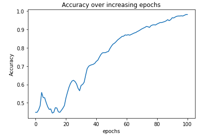
After one epoch
XX = X.cpu().data.numpy()
plt.scatter(XX[:,0],XX[:,1],c=interval_prediction[0])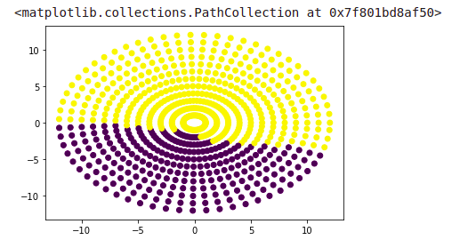
Plots to show performance of neural network over epochs
import matplotlib
matplotlib.use('Agg')
plt.figure(figsize=(16, 32))
for i in range(50):
epoch = i*2 + 2
plt.subplot(10, 5, i+1)
plt.scatter(XX[:,0],XX[:,1],c=interval_prediction[i+1])
plt.title("After {} epochs".format(str(epoch)))
plt.show()
#from matplotlib import pyplot as plt
plt.savefig('epochs.png')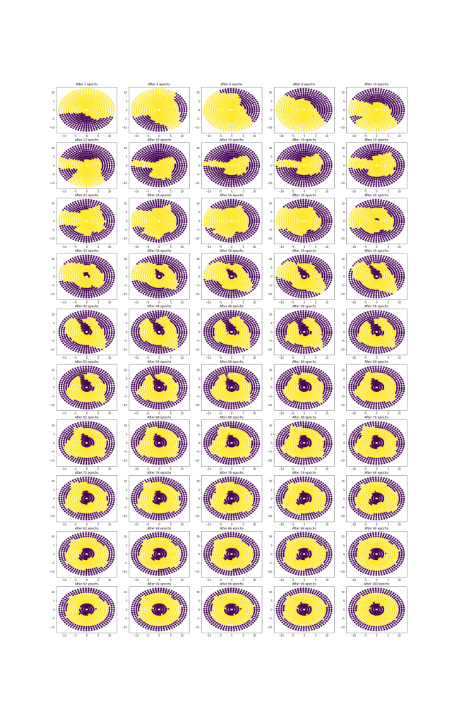

pontu
0
Tags :