Gaussian Double Deep Q Learning
This algorithm extends the traditional Double DQN to handle uncertainties by predicting both the mean and standard deviation of Q-values using a Gaussian distribution. It utilizes KL divergence for the loss function to better measure and minimize the divergence between predicted and target Q-value distributions, providing a more robust approach for reinforcement learning tasks where capturing uncertainty is important.
GaussianDQN
class GaussianDQN(nn.Module):
    def __init__(self, state_dim, action_dim,hidden_dim=256):
        super(GaussianDQN, self).__init__()
        self.fc1 = nn.Linear(state_dim,hidden_dim)
        self.fc2 = nn.Linear(hidden_dim,hidden_dim)
        self.mean_head = nn.Linear(hidden_dim, action_dim)
        self.log_std_head = nn.Linear(hidden_dim, action_dim)

    def forward(self, x):
        x = torch.relu(self.fc1(x))
        x = torch.relu(self.fc2(x))
        mean = self.mean_head(x)
        log_std = self.log_std_head(x)
        std = torch.exp(log_std)
        return mean, std
The GaussianDQN class is a neural network model designed to estimate both the mean and the uncertainty (standard deviation) of Q-values for each action in a reinforcement learning environment. The architecture includes two hidden layers followed by separate output layers for the mean and log standard deviation of the Q-values. This setup allows the model to provide not only the expected Q-values but also a measure of uncertainty, which can be useful for more robust decision-making in uncertain environments.
Loss Function
The compute_loss function calculates the Kullback-Leibler (KL) divergence between two Gaussian distributions. In the context of reinforcement learning, this can be used to measure how one Gaussian distribution (predicted by the model) diverges from another Gaussian distribution (target values).
def compute_loss(pred_mean, pred_std, target_mean, target_std):
    kl_div = torch.log(target_std / pred_std) + (pred_std**2 + (pred_mean - target_mean)**2) / (2 * target_std**2) - 0.5
    return kl_div.mean()
KL Divergence Calculation:
The general formula for the Kullback-Leibler (KL) divergence between two Gaussian distributions p and q is:
(1) 
Log Term
The term that measures the difference in scales (standard deviations) of the two distributions is:
(2) 
Quadratic Term
The term that measures the distance between the predicted mean and variance from the target mean and variance is:
(3) 
Constant Term
The constant term to ensure proper normalization is: 
Action Function
def select_action(state, network, epsilon, action_dim,device):
    if np.random.rand() < epsilon:
        return np.random.randint(action_dim)
    else:
        state = torch.FloatTensor(state).unsqueeze(0).to(device)
        with torch.no_grad():
            mean, _ = network(state)
        return mean.argmax().item()
The select_action function implements an epsilon-greedy policy for action selection in a reinforcement learning setting:
- Exploration: With probability ϵ\epsilonϵ, a random action is chosen to encourage exploring new actions.
- Exploitation: With probability 1−ϵ1 – \epsilon1−ϵ, the action with the highest predicted Q-value (mean) is chosen to exploit the current knowledge for maximizing rewards.
This approach helps balance between trying new actions (which might lead to discovering better strategies) and using the best-known actions to maximize immediate rewards.
Load and Save
These function helps to load and save the model.
def save_checkpoint(state, filename='checkpoint.pth'):
    torch.save(state, filename)
def load_checkpoint(filename='checkpoint.pth', map_location=None):
if map_location:
return torch.load(filename, map_location=map_location)
return torch.load(filename)Hyperparameters and Initialization
Set Device
device = torch.device('cuda' if torch.cuda.is_available() else 'cpu')Set hyperparameters
num_episodes=1000
batch_size=64
gamma=0.99
epsilon_start=1.0
epsilon_end=0.1
epsilon_decay=0.995
epsilon = epsilon_start
update_target_steps = 10000
total_steps = 0
episode_rewards = []
Set the environment and initialize both networks.
env = gym.make("LunarLander-v2")
state_dim = env.observation_space.shape[0]
action_dim = env.action_space.n
hidden_dim = 128

network = GaussianDQN(state_dim, action_dim,hidden_dim).to(device)
target_network = GaussianDQN(state_dim, action_dim,hidden_dim).to(device)
Initialize buffer
replay_buffer = deque(maxlen=100000)Define the optimizer
optimizer = optim.Adam(network.parameters(), lr=0.001)Try to Load the Saved Network
try:
    map_location = torch.device('cpu') if not torch.cuda.is_available() else None
    checkpoint = load_checkpoint(checkpoint_path, map_location=map_location)
    network.load_state_dict(checkpoint['main_net_state_dict'])
    target_network.load_state_dict(checkpoint['target_net_state_dict'])
    optimizer.load_state_dict(checkpoint['optimizer_state_dict'])
    epsilon = checkpoint['epsilon']
    start_episode = checkpoint['episode'] + 1
    print(f"Loaded checkpoint from episode {start_episode}")
except FileNotFoundError:
    print("No checkpoint found, starting from scratch.")
Copy the loaded network to the target network
target_network.load_state_dict(network.state_dict())Train
Initialization and Training Loop
for episode in range(num_episodes):
    state = env.reset()
    episode_reward = 0
for episode in range(num_episodes): Loop through a predefined number of episodes.state = env.reset(): Initialize the environment and get the initial state.episode_reward = 0: Initialize the cumulative reward for the episode.
Inner Loop: Interaction with the Environment
    while True:
        action = select_action(state, network, epsilon, action_dim, device)
        next_state, reward, done, _ = env.step(action)
        replay_buffer.append((state, action, reward, next_state, done))
action = select_action(state, network, epsilon, action_dim, device): Select an action using the epsilon-greedy policy.next_state, reward, done, _ = env.step(action): Execute the action in the environment and observe the next state, reward, and whether the episode is done.replay_buffer.append((state, action, reward, next_state, done)): Store the transition in the replay buffer.
Experience Replay and Network Update
        if len(replay_buffer) > batch_size:
            batch = random.sample(replay_buffer, batch_size)
            states, actions, rewards, next_states, dones = zip(*batch)

            states = torch.FloatTensor(states).to(device)
            actions = torch.LongTensor(actions).to(device)
            rewards = torch.FloatTensor(rewards).to(device)
            next_states = torch.FloatTensor(next_states).to(device)
            dones = torch.FloatTensor(dones).to(device)
if len(replay_buffer) > batch_size: Check if there are enough samples in the replay buffer to form a batch.batch = random.sample(replay_buffer, batch_size): Sample a random batch of transitions from the replay buffer.states, actions, rewards, next_states, dones = zip(*batch): Unpack the batch into separate variables.- Convert these variables into PyTorch tensors and move them to the appropriate device (CPU or GPU).
Compute Predicted and Target Q-Values
            pred_mean, pred_std = network(states)
            pred_mean = pred_mean.gather(1, actions.unsqueeze(1)).squeeze(1)
            pred_std = pred_std.gather(1, actions.unsqueeze(1)).squeeze(1)

            with torch.no_grad():
                next_mean, next_std = target_network(next_states)
                target_mean = rewards + gamma * (1 - dones) * next_mean.max(1)[0]
                target_std = next_std.mean(dim=1)
pred_mean, pred_std = network(states): Get the predicted mean and standard deviation for each state-action pair.pred_mean = pred_mean.gather(1, actions.unsqueeze(1)).squeeze(1): Extract the predicted mean for the taken actions.pred_std = pred_std.gather(1, actions.unsqueeze(1)).squeeze(1): Extract the predicted standard deviation for the taken actions.with torch.no_grad(): Disable gradient calculation for target Q-value computation.next_mean, next_std = target_network(next_states): Get the target network’s predictions for the next states.target_mean = rewards + gamma * (1 - dones) * next_mean.max(1)[0]: Compute the target mean Q-value using the Bellman equation.target_std = next_std.mean(dim=1): Use the mean of the target standard deviations as the target standard deviation.
Compute Loss and Update Network
            loss = compute_loss(pred_mean, pred_std, target_mean, target_std)
            optimizer.zero_grad()
            loss.backward()
            nn.utils.clip_grad_norm_(network.parameters(), 1.0)
            optimizer.step()
loss = compute_loss(pred_mean, pred_std, target_mean, target_std): Compute the loss using the KL divergence between the predicted and target distributions.optimizer.zero_grad(): Clear the gradients from the previous step.loss.backward(): Backpropagate the loss to compute gradients.nn.utils.clip_grad_norm_(network.parameters(), 1.0): Clip gradients to prevent exploding gradients.optimizer.step(): Update the network parameters using the computed gradients.
Episode End Handling and Target Network Update
        state = next_state
        episode_reward += reward
        total_steps += 1

        if done:
            break

        if total_steps % update_target_steps == 0:
            target_network.load_state_dict(network.state_dict())
state = next_state: Move to the next state.episode_reward += reward: Accumulate the episode reward.total_steps += 1: Increment the total steps counter.if done: break: Break the loop if the episode is done.if total_steps % update_target_steps == 0:- Update the target network periodically by copying the weights from the main network.
Epsilon Decay, Logging, and Checkpointing
    epsilon = max(epsilon_end, epsilon * epsilon_decay)
    episode_rewards.append(episode_reward)
    print(f"Episode {episode + 1}, Reward: {episode_reward}, Epsilon: {epsilon:.2f}")

    if episode % 50 == 0:
        save_checkpoint({
            'episode': episode,
            'main_net_state_dict': network.state_dict(),
            'target_net_state_dict': target_network.state_dict(),
            'optimizer_state_dict': optimizer.state_dict(),
            'epsilon': epsilon
        }, checkpoint_path)
        print(f"Checkpoint saved at episode {episode}")

    if sum(episode_rewards[-5:]) > 1000:
        print(sum(episode_rewards[-5:]) > 1000)
        print("Training done")
        save_checkpoint({
            'episode': episode,
            'main_net_state_dict': network.state_dict(),
            'target_net_state_dict': target_network.state_dict(),
            'optimizer_state_dict': optimizer.state_dict(),
            'epsilon': epsilon
        }, checkpoint_path)
        print(f"Checkpoint saved at episode {episode}")
        break
epsilon = max(epsilon_end, epsilon * epsilon_decay): Decay the epsilon value to reduce exploration over time.episode_rewards.append(episode_reward): Log the episode reward.print(f"Episode {episode + 1}, Reward: {episode_reward}, Epsilon: {epsilon:.2f}"): Print the episode’s statistics.- Periodically save a checkpoint of the model:
- If the sum of the rewards over the last 5 episodes exceeds 1000, save a final checkpoint and stop training:
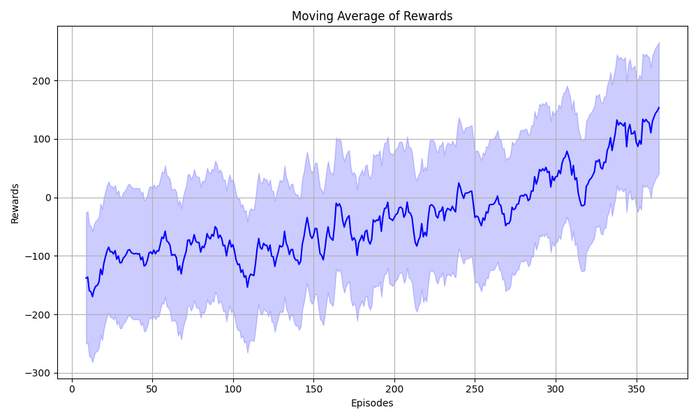
Plot the Progress
import pandas as pd
import numpy as np
import seaborn as sns
import matplotlib.pyplot as plt

# Generate some sample data
np.random.seed(0)
data = episode_rewards

# Calculate the moving average
window_size = 10
moving_avg = pd.Series(data).rolling(window=window_size).mean()

# Plotting
plt.figure(figsize=(10, 6))

# Plot the moving average line
sns.lineplot(data=moving_avg, color='blue')

# Shade the area around the moving average line to represent the range of values
plt.fill_between(range(len(moving_avg)),
                 moving_avg - np.std(data),
                 moving_avg + np.std(data),
                 color='blue', alpha=0.2)

plt.xlabel('Episodes')
plt.ylabel('Rewards')
plt.title('Moving Average of Rewards')
plt.grid(True)
# Adjust layout to prevent overlapping elements
plt.tight_layout()

# Save the plot as a PNG file
plt.savefig('Episode_rewards.png')
# Show the plot
plt.show()