Azure MLOps for Beginners: Train, Deploy and Serve a GRU forecasting model.

Azure MLOps for Begineers is two part tutorial, where we will learn to create a fully operational pipeline using AzureML, GRU deep learning and Flask, enabling us to go from raw stock data to production ready forecasting – all in the Azure.

In this first part, we will fetch data, train the GRU model on Azure, register the model and deploy the model as a REST endpoint.

The Setup

Create a directory in your local machine along with virtual python environment.

mkdir Azure_GRU
cd Azure_GRU
python3 -m venv venv
source venv/bin/activate

Launch the Azure Machine Learning studio. After launching, click on top right. You will see the basic information: your resource group, subscription id etc. along with the link to download config file. Download the config file and move it the your current working folder in your local setup.

The Files

helper.py

Create a helper.py file in the same folder. This file will contain all the necessary functions to get the data from API and convert it to dataframe, convert the data from dataframe to a specific shape suitable for training, a function to normalize data and a function to train and evaluate model. This file also contains a Class to define GRU model.

import torch
import torch.nn as nn
import numpy as np
import pandas as pd
from datetime import datetime, timedelta
from matplotlib import pyplot as plt
from sklearn.preprocessing import StandardScaler
from sklearn.metrics import mean_absolute_percentage_error
from azureml.core import Run




#function to load data from api
def custom_business_week_mean(values):
    # Filter out Saturdays
    working_days = values[values.index.dayofweek != 5]
    return working_days.mean()

#function to read stock data from Nepalipaisa.com api
def stock_dataFrame(stock_symbol,start_date='2020-01-01',weekly=False):
  """
  input : stock_symbol
            start_data set default at '2020-01-01'
            weekly set default at False
  output : dataframe of daily or weekly transactions
  """
  #print(end_date)
  today = datetime.today()
  # Calculate yesterday's date
  yesterday = today - timedelta(days=1)

  # Format yesterday's date
  formatted_yesterday = yesterday.strftime('%Y-%-m-%-d')
  print(formatted_yesterday)


  path = f'https://www.nepalipaisa.com/api/GetStockHistory?stockSymbol={stock_symbol}&fromDate={start_date}&toDate={formatted_yesterday}&pageNo=1&itemsPerPage=10000&pagePerDisplay=5&_=1686723457806'
  df = pd.read_json(path)
  theList = df['result'][0]
  df = pd.DataFrame(theList)
  #reversing the dataframe
  df = df[::-1]

  #removing 00:00:00 time
  #print(type(df['tradeDate'][0]))
  df['Date'] = pd.to_datetime(df['tradeDateString'])

  #put date as index and remove redundant date columns
  df.set_index('Date', inplace=True)
  columns_to_remove = ['tradeDate', 'tradeDateString','sn']
  df = df.drop(columns=columns_to_remove)

  new_column_names = {'maxPrice': 'High', 'minPrice': 'Low', 'closingPrice': 'Close','volume':'Volume','previousClosing':"Open"}
  df = df.rename(columns=new_column_names)

  if(weekly == True):
     weekly_df = df.resample('W').apply(custom_business_week_mean)
     df = weekly_df


  return df


def create_sequences(df, window_size=5):
    """
    Create input-output sequences for time series forecasting.
    
    Parameters:
    - df: pandas DataFrame with 'Close' column
    - window_size: number of days to use as input (default 5)
    
    Returns:
    - X: numpy array of shape (n_samples, window_size) containing input sequences
    - y: numpy array of shape (n_samples,) containing target prices
    """
    close_prices = df['Close'].values
    X = []
    y = []
    
    # Create sliding windows
    for i in range(len(close_prices) - window_size):
        # Get the window of features
        window = close_prices[i:i+window_size]
        X.append(window)
        
        # Get the target (next day's close)
        target = close_prices[i+window_size]
        y.append(target)
    
    return np.array(X), np.array(y)

def normalize_data(X, y):
    """
    Normalize input sequences and target values using StandardScaler.
    
    Parameters:
    - X: Input sequences (n_samples, window_size)
    - y: Target values (n_samples,)
    
    Returns:
    - X_scaled: Normalized input sequences
    - y_scaled: Normalized target values
    - scaler: Fitted scaler object for inverse transformation
    """
    # Reshape X to 2D (n_samples * window_size, 1) for scaling
    X_reshaped = X.reshape(-1, 1)
    
    # Initialize and fit scaler
    scaler = StandardScaler()
    X_scaled = scaler.fit_transform(X_reshaped)
    
    # Reshape back to original shape
    X_scaled = X_scaled.reshape(X.shape)
    
    # Scale target values using the same scaler
    y_scaled = scaler.transform(y.reshape(-1, 1)).flatten()
    
    return X_scaled, y_scaled, scaler


    
class GRUModel(nn.Module):
    
    def __init__(self,input_size,hidden_size,output_size):
        super(GRUModel,self).__init__()
        self.gru = nn.GRU(input_size,hidden_size,batch_first=True)
        self.fc = nn.Linear(hidden_size,output_size)
        
    def forward(self,x):
        _,h_n = self.gru(x)
        return self.fc(h_n.squeeze(0))

    

def train_and_evaluate_gru(X_train, y_train, X_test, y_test, input_size=1, hidden_size=32, output_size=1, epochs=100, lr=0.001):
    model = GRUModel(input_size, hidden_size, output_size)
    criterion = nn.MSELoss()
    optimizer = torch.optim.Adam(model.parameters(), lr=lr)

    train_losses = []
    test_losses = []
    test_mapes = []

    for epoch in range(epochs):
        print(f"Epoch no: {epoch+1}")
        model.train()
        train_preds = model(X_train)
        loss = criterion(train_preds.squeeze(), y_train)

        optimizer.zero_grad()
        loss.backward()
        optimizer.step()

        model.eval()
        with torch.no_grad():
            test_preds = model(X_test)
            test_loss = criterion(test_preds.squeeze(), y_test)
            test_mape = mean_absolute_percentage_error(y_test.numpy(), test_preds.squeeze().numpy())
            
            
        train_losses.append(loss.item())
        test_losses.append(test_loss.item())
        test_mapes.append(test_mape)

        if epoch % 10 == 0 or epoch == epochs - 1:
            print(f"Epoch {epoch:03d}: Train Loss={loss.item():.4f}, Test Loss={test_loss.item():.4f}, Test MAPE={test_mape:.2f}%")

    return model, train_losses, test_losses, test_mapes

train.py

Create another file, train.py. This file will use the functions of helper.py to get data and train the model. I will also register the model and the scalar of the data after training. Apart form registering models, it will also save logs and plots.

import torch
import argparse
import os
import joblib
from azureml.core import Run, Model
import matplotlib.pyplot as plt
from sklearn.model_selection import train_test_split
from helper import stock_dataFrame,create_sequences,normalize_data,train_and_evaluate_gru


# # Get Azure ML Run context
run = Run.get_context()
# Parse hyperparameters
parser = argparse.ArgumentParser()
parser.add_argument("--symbol",type=str,default="ADBL",help="The stock symbol")
parser.add_argument("--epochs", type=int, default=10, help="Number of training epochs")
parser.add_argument("--input_size",type=int,default=1,help="input size")
parser.add_argument("--hidden_size",type=int,default=32,help="hidden size")
parser.add_argument("--output_size",type=int,default=1,help="output size")
args = parser.parse_args()

#1. Get the data
stock_symbol = args.symbol
df = stock_dataFrame(stock_symbol,start_date='2020-01-01',weekly=False)
df = df[['Close']]
df.dropna(inplace=True)

#2. Format the data 
X,y = create_sequences(df, window_size=5)

# 3. Normalize data
X_scaled, y_scaled, scaler = normalize_data(X, y)

# 4. Reshape for GRU (samples, timesteps, features)
X_scaled = X_scaled.reshape(X_scaled.shape[0], X_scaled.shape[1], 1)

# 5. Split into train/test
X_train, X_test, y_train, y_test = train_test_split(
    X_scaled, y_scaled, test_size=0.2, shuffle=False)

# 6. Convert to PyTorch tensors
X_train = torch.FloatTensor(X_train)
y_train = torch.FloatTensor(y_train)
X_test = torch.FloatTensor(X_test)
y_test = torch.FloatTensor(y_test)

print(f"Shape of X_train: {X_train.shape}")
print(f"Shape of y_train: {y_train.shape}")

 # 6. Train model
model, train_losses, test_losses, test_mapes = train_and_evaluate_gru(X_train, y_train, X_test, y_test, input_size=1, hidden_size=32, output_size=1, epochs=100, lr=0.001)
print("Test_MAPE",sum(test_mapes)/len(test_mapes))
run.log("Test_MAPE",sum(test_mapes)/len(test_mapes))

# 7. save model
os.makedirs("outputs",exist_ok=True)
model_path = "outputs/pytorch_nn_gru.pth"
torch.save(model.state_dict(),model_path)
print(f"Model saved in {model_path}")
# #register model
Model.register(
    workspace=run.experiment.workspace,
    model_name="pytorch_nn_gru",
    model_path = model_path,
    description="adbl trained on new gru"
)
print("Model registered successfully")


# 8. Save scaler
scaler_path = "outputs/scaler_adbl.save"
joblib.dump(scaler, scaler_path)
print(f"Scaler saved at {scaler_path}")

# Register scaler
Model.register(
    workspace=run.experiment.workspace,
    model_name="adbl_scaler",
    model_path=scaler_path,
    description="Scaler used for ADBL GRU model"
)
print("Scaler registered successfully")


# # 7. Plot results
plt.figure(figsize=(10, 5))
plt.plot(train_losses, label='Train LOSSES')
plt.plot(test_losses, label='Test LOSSES')
plt.title('LOSS Over Epochs')
plt.xlabel('Epoch')
plt.ylabel('LOSS (%)')
plt.legend()
plt.show()
# Save the plot to a file
plot_path = "LOSS.png"
plt.savefig(plot_path)
plt.close()
# Log the plot to Azure ML
run.log_image('LOSS PLOT', plot_path)


# Complete run
run.complete()

environment.yml

Now, create a file named environment.yml

name: pytorch-env
dependencies:
  - python=3.10
  - pytorch=2.1.0
  - scikit-learn
  - pip
  - pip:
      - azureml-sdk
      - mlflow
      - numpy
      - matplotlib
      - pandas

This files defines a reproducible environment for training and deploying machine learning models – in this case, using the PyTorch and Azure ML.

This files specifies the conda environment configuration that Azure ML (or local tools like conda) can use to:

• Recreate a consistent environment across training, testing and deployment.
• Package and deploy your model in a container with all the dependencies it needs.

It ensures portability, reproducibility and compatibility – core principles of MLops.

• name: pytorch-env
  • This gives the environment a name. We can refer to this name when activating or referencing it within Azure ML or locally.
• depencencies:
  • This section lists everything the environment need to function, like python, pytorch, scikit-learn, pip.
• pip:
  • This sublist includes Python Packages that will be installed via pip.

Conda first installs the core environments (Python, Pytorch, scikit-learn), then pip installs additional packages into the environment. Azure ML builds this in order, ensuring dependencies do not clash.

Create, train, save and register

run.ipynb

from azureml.core import Workspace, Experiment, ScriptRunConfig, Environment

# Connect to Azure ML Workspace
ws = Workspace.from_config()  # Ensure your `config.json` file is present

# Create an Azure ML experiment
experiment = Experiment(ws, "Pytorch-NN-GRU")

# Define an execution environment
env = Environment.from_conda_specification(name="pytorch-env", file_path="environment.yml")

Above code connects to the Azure ML Workspace, create an Azure ML experiment and an execution environment with the help of “environment.yml” file.

from azureml.core.compute import ComputeInstance, ComputeTarget
from azureml.exceptions import ComputeTargetException



# Define compute instance name
compute_name = "compute-A42"

# Set VM size (adjust as needed)
vm_size = "Standard_DS3_v2"

try:
    # Check if the compute instance already exists
    compute_instance = ComputeInstance(ws, compute_name)
    print(f"Compute instance {compute_name} already exists.")

except ComputeTargetException:
    print(f"Creating new compute instance: {compute_name}")

    compute_config = ComputeInstance.provisioning_configuration(vm_size=vm_size)

    compute_instance = ComputeInstance.create(ws, compute_name, compute_config)
    compute_instance.wait_for_completion(show_output=True)

print(f"Compute instance '{compute_name}' is ready!")

This creates a new compute instance in your Azure with compute name “compute-A42”.

# Set up the script configuration
compute_name = "compute-A42"
script_config = ScriptRunConfig(
    source_directory=".",  # Path to the script folder
    script="train.py",  
    compute_target=compute_name,  # Change to your Azure ML compute name
    environment=env,
    arguments=["--symbol","ADBL","--input_size",1,"--hidden_size",32,"--output_size",1,"--epochs", 200]
)

This script sets up a training job using Azure ML’s ScriptRunConfig.
It specifies the script location (train.py), compute target (compute-A42), and environment (env).
Custom arguments like stock symbol, model parameters, and epochs are passed in.
This configuration is used to submit and run training remotely on Azure.

# Submit experiment
run = experiment.submit(script_config)
print("Experiment submitted! Tracking in Azure ML Studio.")
run.wait_for_completion(show_output=True)

This code submits the training job to Azure ML for execution.
It tracks the run under the specified experiment and provides a live output of training progress.
run.wait_for_completion(show_output=True) blocks the script until the run finishes.
You can monitor the run details, logs, and metrics in Azure ML Studio.

Check Azure

Go to home page of your Azure ML studio. On left under assets you will find jobs, models etc.

Let’s check jobs.

Click on the latest job or the job just completed.

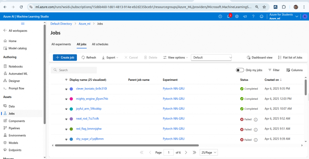
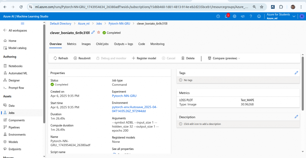
You can check metrics, images and others.

Now, again from left, select models.

You will see your model and scalar. Code to register both models and scaler along with the metrics and images were written in train.py

Now, after training the model and registering it successfully, we will deploy it.

Deployment

score.py

score.py is what lets your model work in production. It tells Azure ML how to use your model once it’s deployed—making it a core piece of any ML deployment pipeline.

import json
import torch
import torch.nn as nn
import numpy as np
import os
import joblib
from azureml.core.model import Model


class GRUModel(nn.Module):
    def __init__(self, input_size, hidden_size, output_size):
        super(GRUModel, self).__init__()
        self.gru = nn.GRU(input_size, hidden_size, batch_first=True)
        self.fc = nn.Linear(hidden_size, output_size)

    def forward(self, x):
        _, h_n = self.gru(x)
        return self.fc(h_n.squeeze(0))


# Global model and scaler objects
model = None
scaler = None


def init():
    global model, scaler

    # Load GRU model
    model_path = Model.get_model_path("pytorch_nn_gru")
    model = GRUModel(input_size=1, hidden_size=32, output_size=1)
    model.load_state_dict(torch.load(model_path, map_location=torch.device("cpu")))
    model.eval()

    # Load scaler
    scaler_path = Model.get_model_path("adbl_scaler")
    scaler = joblib.load(scaler_path)


def run(raw_data):
    try:
        data = json.loads(raw_data)
        inputs = data["data"]  # expects [[val1, val2, val3, val4, val5], ...]

        # Convert to tensor with shape (batch_size, 5, 1)
        x = torch.tensor(inputs, dtype=torch.float32).unsqueeze(-1)

        with torch.no_grad():
            predictions = model(x)

        preds_np = predictions.numpy().reshape(-1, 1)

        # Inverse transform using the scaler if y was scaled
        preds_inversed = scaler.inverse_transform(preds_np)

        return preds_inversed.flatten().tolist()

    except Exception as e:
        return {"error": str(e)}

Azure ML endpoints call score.py when receiving a prediction request.

It contains two required functions:

• init() – loads your model and any necessary artifacts (e.g., scalers).
• run() – takes incoming data, runs inference, and returns the result.

deployment.ipynb

from azureml.core import Environment

env = Environment(name="azure_pytorch_env")
env.python.conda_dependencies.add_pip_package("torch==2.1.0")
env.python.conda_dependencies.add_pip_package("numpy")
env.python.conda_dependencies.add_pip_package("scikit-learn")

This code creates a custom Azure ML environment named "azure_pytorch_env" and installs PyTorch 2.1.0, NumPy, and scikit-learn via pip. It’s used to ensure consistent dependencies during model training and deployment.

from azureml.core import Workspace, Model
from azureml.core.webservice import AciWebservice
from azureml.core.model import InferenceConfig

# Connect to Azure ML Workspace
ws = Workspace.from_config()

# Load registered model and scaler
model = Model(ws, "pytorch_nn_gru")
scaler = Model(ws, "adbl_scaler")


# Define inference configuration
inference_config = InferenceConfig(
    entry_script="score.py",
    environment=env
)

# Define deployment configuration (ACI)
deployment_config = AciWebservice.deploy_configuration(cpu_cores=1, memory_gb=1)

# Deploy both the model and scaler
service = Model.deploy(
    workspace=ws,
    name="pytorch-n-gru-scalar",
    models=[model, scaler],  # <-- Include both
    inference_config=inference_config,
    deployment_config=deployment_config
)

service.wait_for_deployment(show_output=True)

# Print Scoring URI
print(f"Deployment successful! Scoring URI: {service.scoring_uri}")

1. Connect to Workspace & Load Models:
   Connects to Azure ML workspace using config file.
   Loads both the GRU model and the corresponding scaler registered in Azure.
2. Define Inference Configuration:
   Specifies the score.py script for inference logic.
   Defines the environment with necessary packages for deployment.
3. Define Deployment Configuration:
   Sets up deployment target as Azure Container Instance (ACI).
   Allocates 1 CPU core and 1GB memory for the deployed service.
4. Deploy the Model & Scaler:
   Deploys both model and scaler together as a web service.
   Waits for deployment completion and displays output logs.
5. Output the Scoring URI:
   Prints the URI endpoint to interact with the deployed model.
   This URI is used by applications (like Flask) to send requests.

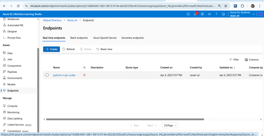
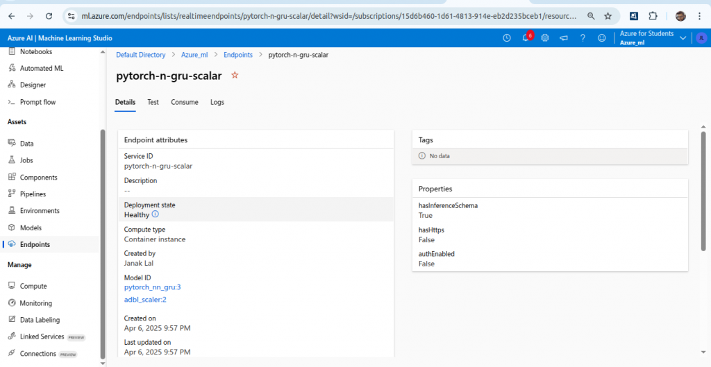
After completion of this, you can see your endpoint in Azure ML.

Test the deployed endpoint with the following code.

import requests
import json

# Select a sample (first one for testing)

sample_input = [[0.1, 0.2, 0.3, 0.4, 0.5],
        [0.5, 0.4, 0.3, 0.2, 0.1]]

# Define the input JSON payload
payload = json.dumps({"data": sample_input})

# Get the deployment endpoint
scoring_uri = service.scoring_uri
headers = {"Content-Type": "application/json"}

# Send request to the deployed model
response = requests.post(scoring_uri, data=payload, headers=headers)

# Print response
print("Response:", response.json())

Output

Response: [385.9725646972656, 385.8465270996094]

Conclusion

In this part we learnt to train, register and deploy our model. In next part, we will learn how to create a flask web application which will use this endpoint to forecast the stock price.

You can find all the codes in github.