U²-Net with PyTorch: Salient Object Detection and Background Removal Tutorial
Learn how to implement U²-Net with PyTorch for salient object detection and background removal. Step-by-step guide with code examples and explanations.
Table of Contents
- Introduction to U²-Net
- ECSSD Dataset
- Import
- Data Preparation
- The U²-Net
- The Loss Function
- Initialization
- Training
- Plotting The Losses and IOU
- Results
- Background Removal
- Github and Streamlit Link
Introduction to U²-Net:
Salient Object Detection (SOD) aims at segmenting the most visually attractive objects in an image. It is widely used in many fields, such as visual tracking and image segmentation.
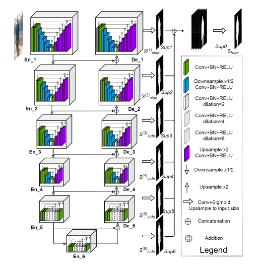
U²-Net is a two-level nested U-structure that is designed for SOD without using any pre-trained backbones from image classification. It can be trained from scratch to achieve competitive performance. Second, this architecture allows the network to go deeper, attain high resolution, without significantly increasing the memory and computation cost. This is achieved by a nested U-structure: on the bottom level, where a ReSidual U-block is able to extract intra-stage multi-scale features without degrading the feature map resolution; on the top level, there is a U-Net like structure, in which each stage is filled by a RSU block. The two level configuration results in a nested U-structure.
For more theoretical detail on U²-Net read this original paper.
ECSSD Dataset
The Extended Complex Scene Saliency Dataset (ECSSD) is a widely used benchmark for salient object detection, containing 1,000 natural images with diverse and cluttered backgrounds along with pixel-level ground truth masks. Introduced by Jianming Zhang et al. in 2013, the dataset was designed to challenge saliency detection models by including complex scenes where salient objects are not easily distinguishable from the background. ECSSD is frequently used to evaluate models like U²-Net, as it provides a reliable testbed for assessing robustness and accuracy in real-world scenarios.
Download the image and the mask of ECSSD dataset using the following code.
!wget http://www.cse.cuhk.edu.hk/leojia/projects/hsaliency/data/ECSSD/images.zip
!wget http://www.cse.cuhk.edu.hk/leojia/projects/hsaliency/data/ECSSD/ground_truth_mask.zip
Unzip the data.
!unzip images.zip
!unzip ground_truth_mask.zip
Move to the required folder if necessary.
!mv /content/images/* "/ECSSD_Dataset/Images"
!mv/content/ground_truth_mask/*"/ECSSD_Dataset/Masks"
Import necessary Libraries
import os
import random

import numpy as np
import matplotlib.pyplot as plt
from PIL import Image

import torch
import torch.nn as nn
import torch.nn.functional as F
import torch.optim as optim

from torch.utils.data import Dataset, DataLoader
from torchvision import transforms

from tqdm import tqdm
from google.colab import files
Data Preparation
Define the directory of images and masks
image_dir = "/ECSSD_Dataset/Images"
mask_dir = "/ECSSD_Dataset/Masks"
Dataset Class
It is an abstract class that represents a dataset. Its main function is to provide a standard way to access and manage data samples so they can be easily used in training or testing machine learning models.
The main function of this Dataset class are as follows:
- Data Wrapping: It lets us wrap our dataset (images, text, tabular data, etc.) into a Python object. Instead of using a raw arrays, we use a Dataset object.
- Indexing Access (__getitem__): We can access a single data sample (and its label, if supervised) using an index.
- Dataset Length (__len__): This method tells Python how many samples the dataset contains.
- Integration with Dataloader: A dataset is usually passed to a DataLoader which handles Batching, Shuffling and Parallel Loading.
For our purpose we created a ECSSDataset class, which is a custom Pytorch dataset for handling the ECSSD saliency dataset. It takes two directories: one containing images (.jpg) and the other containing ground truth-masks (.png). The class ensures that each image has a corresponding mask and allows optional data augmentations (like resizing, flipping, etc) to be applied consistently to both image and mask.
This makes dataset ready to be used with a PyTorch DataLoader for training segmentation models.
# Custom Dataset Class with Augmentation
class ECSSDDataset(Dataset):
    def __init__(self, image_dir, mask_dir, transform=None, train=True):
        self.image_dir = image_dir
        self.mask_dir = mask_dir
        self.train = train
        self.transform = transform
        self.image_files = sorted([f for f in os.listdir(image_dir) if f.endswith('.jpg')])
        self.mask_files = sorted([f for f in os.listdir(mask_dir) if f.endswith('.png')])

        # Verify matching pairs
        assert len(self.image_files) == len(self.mask_files)
        for img, mask in zip(self.image_files, self.mask_files):
            assert os.path.splitext(img)[0] == os.path.splitext(mask)[0]

    def __len__(self):
        return len(self.image_files)

    def __getitem__(self, idx):
        img_path = os.path.join(self.image_dir, self.image_files[idx])
        mask_path = os.path.join(self.mask_dir, self.mask_files[idx])

        image = Image.open(img_path).convert('RGB')
        mask = Image.open(mask_path).convert('L')  # Convert to grayscale

        if self.transform:
            seed = torch.random.seed()

            # Apply same transform to both image and mask
            torch.random.manual_seed(seed)
            image = self.transform(image)

            torch.random.manual_seed(seed)
            mask = self.transform(mask)

        return image, mask
Now we define two different transformation pipelines are defined: one with data augmentation for training (resizing, random flips, rotations, color jittering, and tensor conversion) and another simpler one for validation/testing (just resizing and tensor conversion). The custom ECSSDDataset class is then used to create train_dataset and test_dataset, applying the appropriate transforms. Finally, PyTorch DataLoaders are set up: the training loader shuffles data for better generalization, while the test loader keeps the order fixed. Both loaders use batching (batch_size=8), multiple workers (num_workers=4) for faster data loading, and pin_memory=True for efficient transfer to the GPU.
# Define transformations with augmentation for training
train_transform = transforms.Compose([
    transforms.Resize((320, 320)),
    transforms.RandomHorizontalFlip(p=0.5),
    transforms.RandomVerticalFlip(p=0.5),
    transforms.RandomRotation(15),
    transforms.ColorJitter(brightness=0.2, contrast=0.2),
    transforms.ToTensor(),
])

# Simpler transform for validation
val_transform = transforms.Compose([
    transforms.Resize((320, 320)),
    transforms.ToTensor(),
])

# Create datasets
train_dataset = ECSSDDataset(image_dir, mask_dir, transform=train_transform, train=True)
test_dataset = ECSSDDataset(image_dir, mask_dir, transform=val_transform, train=False)

# Create dataloaders
train_loader = DataLoader(train_dataset, batch_size=8, shuffle=True, num_workers=4, pin_memory=True)
test_loader = DataLoader(test_dataset, batch_size=8, shuffle=False, num_workers=4, pin_memory=True)
U²-Net with PyTorch
REBNCONV
REBNCONV is the basic convolutional building block used everywhere in this U²-Net code.
Concretely it does:
- a 3×3
Conv2d(mapsin_ch→out_ch) withdilation=dirateandpadding=dirate(so spatial size is preserved while the receptive field can be increased), BatchNorm2dto stabilize and speed up training,ReLU(inplace=True)for nonlinearity and memory efficiency.
It returns the activated feature map (conv → bn → relu).
class REBNCONV(nn.Module):
    def __init__(self,in_ch=3,out_ch=3,dirate=1):
        super(REBNCONV,self).__init__()

        self.conv_s1 = nn.Conv2d(in_ch,out_ch,3,padding=1*dirate,dilation=1*dirate)
        self.bn_s1 = nn.BatchNorm2d(out_ch)
        self.relu_s1 = nn.ReLU(inplace=True)

    def forward(self,x):

        hx = x
        xout = self.relu_s1(self.bn_s1(self.conv_s1(hx)))

        return xout
_upsample_like
_upsample_like(src, tar) ensures tensors align spatially so concatenation and elementwise operations can work correctly.
RSU7
RSU7 stands for Residual U-block with 7 stages.
It’s one of the encoder–decoder style building blocks used inside U²-Net.
Each RSU block looks like a mini U-Net inside a bigger U-Net, where features go through multiple downsampling (via pooling), bottleneck layers with dilation, and then symmetric upsampling back, with skip connections at every level.
The purpose of RSU7 is to capture multi-scale contextual information while preserving spatial detail through skip connections and residual learning (return hx1d + hxin).
The structure of RSU7:
- Input Convolution (
rebnconvin):Brings input into a consistent feature space (in_ch → out_ch). - Encoder Path (6 steps)
rebnconv1→ feature extractionpool1→ downsamplerebnconv2,rebnconv3,rebnconv4,rebnconv5,rebnconv6with intermediate pooling- progressively reduces spatial size, increases receptive field.
- Bottom Layer (
rebnconv7): Uses a dilated convolution to capture global context without reducing resolution further. - Decoder Path
- Starts from the bottleneck (
hx7) - Concatenates with encoder features (
torch.cat) - Upsamples step by step (
_upsample_like) - Refines features (
rebnconv6d,rebnconv5d, …,rebnconv1d).
- Starts from the bottleneck (
- Residual Output: Final output is
hx1d + hxin, meaning the block learns a residual mapping on top of the input features.
class RSU7(nn.Module):#UNet07DRES(nn.Module):

    def __init__(self, in_ch=3, mid_ch=12, out_ch=3):
        super(RSU7,self).__init__()

        self.rebnconvin = REBNCONV(in_ch,out_ch,dirate=1)

        self.rebnconv1 = REBNCONV(out_ch,mid_ch,dirate=1)
        self.pool1 = nn.MaxPool2d(2,stride=2,ceil_mode=True)

        self.rebnconv2 = REBNCONV(mid_ch,mid_ch,dirate=1)
        self.pool2 = nn.MaxPool2d(2,stride=2,ceil_mode=True)

        self.rebnconv3 = REBNCONV(mid_ch,mid_ch,dirate=1)
        self.pool3 = nn.MaxPool2d(2,stride=2,ceil_mode=True)

        self.rebnconv4 = REBNCONV(mid_ch,mid_ch,dirate=1)
        self.pool4 = nn.MaxPool2d(2,stride=2,ceil_mode=True)

        self.rebnconv5 = REBNCONV(mid_ch,mid_ch,dirate=1)
        self.pool5 = nn.MaxPool2d(2,stride=2,ceil_mode=True)

        self.rebnconv6 = REBNCONV(mid_ch,mid_ch,dirate=1)

        self.rebnconv7 = REBNCONV(mid_ch,mid_ch,dirate=2)

        self.rebnconv6d = REBNCONV(mid_ch*2,mid_ch,dirate=1)
        self.rebnconv5d = REBNCONV(mid_ch*2,mid_ch,dirate=1)
        self.rebnconv4d = REBNCONV(mid_ch*2,mid_ch,dirate=1)
        self.rebnconv3d = REBNCONV(mid_ch*2,mid_ch,dirate=1)
        self.rebnconv2d = REBNCONV(mid_ch*2,mid_ch,dirate=1)
        self.rebnconv1d = REBNCONV(mid_ch*2,out_ch,dirate=1)

    def forward(self,x):

        hx = x
        hxin = self.rebnconvin(hx)

        hx1 = self.rebnconv1(hxin)
        hx = self.pool1(hx1)

        hx2 = self.rebnconv2(hx)
        hx = self.pool2(hx2)

        hx3 = self.rebnconv3(hx)
        hx = self.pool3(hx3)

        hx4 = self.rebnconv4(hx)
        hx = self.pool4(hx4)

        hx5 = self.rebnconv5(hx)
        hx = self.pool5(hx5)

        hx6 = self.rebnconv6(hx)

        hx7 = self.rebnconv7(hx6)

        hx6d =  self.rebnconv6d(torch.cat((hx7,hx6),1))
        hx6dup = _upsample_like(hx6d,hx5)

        hx5d =  self.rebnconv5d(torch.cat((hx6dup,hx5),1))
        hx5dup = _upsample_like(hx5d,hx4)

        hx4d = self.rebnconv4d(torch.cat((hx5dup,hx4),1))
        hx4dup = _upsample_like(hx4d,hx3)

        hx3d = self.rebnconv3d(torch.cat((hx4dup,hx3),1))
        hx3dup = _upsample_like(hx3d,hx2)

        hx2d = self.rebnconv2d(torch.cat((hx3dup,hx2),1))
        hx2dup = _upsample_like(hx2d,hx1)

        hx1d = self.rebnconv1d(torch.cat((hx2dup,hx1),1))

        return hx1d + hxin
This design helps the network extract multi-scale, context-rich features while avoiding loss of fine spatial details.
RSU6, RSU5, and RSU4 are progressively shallower variants of the RSU7 block, following the same encoder–decoder design with residual connections but with fewer downsampling/upsampling stages.
RSU4F is a special “flat” variant of RSU4 that removes all pooling and upsampling operations. Instead, it stacks multiple dilated convolutions with increasing dilation rates (1, 2, 4, 8) to directly expand the receptive field while keeping spatial resolution constant. This makes RSU4F especially useful for the deepest layers of U²-Net, where global context is needed but spatial alignment with skip connections must be preserved.
### RSU-6 ###
class RSU6(nn.Module):#UNet06DRES(nn.Module):

    def __init__(self, in_ch=3, mid_ch=12, out_ch=3):
        super(RSU6,self).__init__()

        self.rebnconvin = REBNCONV(in_ch,out_ch,dirate=1)

        self.rebnconv1 = REBNCONV(out_ch,mid_ch,dirate=1)
        self.pool1 = nn.MaxPool2d(2,stride=2,ceil_mode=True)

        self.rebnconv2 = REBNCONV(mid_ch,mid_ch,dirate=1)
        self.pool2 = nn.MaxPool2d(2,stride=2,ceil_mode=True)

        self.rebnconv3 = REBNCONV(mid_ch,mid_ch,dirate=1)
        self.pool3 = nn.MaxPool2d(2,stride=2,ceil_mode=True)

        self.rebnconv4 = REBNCONV(mid_ch,mid_ch,dirate=1)
        self.pool4 = nn.MaxPool2d(2,stride=2,ceil_mode=True)

        self.rebnconv5 = REBNCONV(mid_ch,mid_ch,dirate=1)

        self.rebnconv6 = REBNCONV(mid_ch,mid_ch,dirate=2)

        self.rebnconv5d = REBNCONV(mid_ch*2,mid_ch,dirate=1)
        self.rebnconv4d = REBNCONV(mid_ch*2,mid_ch,dirate=1)
        self.rebnconv3d = REBNCONV(mid_ch*2,mid_ch,dirate=1)
        self.rebnconv2d = REBNCONV(mid_ch*2,mid_ch,dirate=1)
        self.rebnconv1d = REBNCONV(mid_ch*2,out_ch,dirate=1)

    def forward(self,x):

        hx = x

        hxin = self.rebnconvin(hx)

        hx1 = self.rebnconv1(hxin)
        hx = self.pool1(hx1)

        hx2 = self.rebnconv2(hx)
        hx = self.pool2(hx2)

        hx3 = self.rebnconv3(hx)
        hx = self.pool3(hx3)

        hx4 = self.rebnconv4(hx)
        hx = self.pool4(hx4)

        hx5 = self.rebnconv5(hx)

        hx6 = self.rebnconv6(hx5)


        hx5d =  self.rebnconv5d(torch.cat((hx6,hx5),1))
        hx5dup = _upsample_like(hx5d,hx4)

        hx4d = self.rebnconv4d(torch.cat((hx5dup,hx4),1))
        hx4dup = _upsample_like(hx4d,hx3)

        hx3d = self.rebnconv3d(torch.cat((hx4dup,hx3),1))
        hx3dup = _upsample_like(hx3d,hx2)

        hx2d = self.rebnconv2d(torch.cat((hx3dup,hx2),1))
        hx2dup = _upsample_like(hx2d,hx1)

        hx1d = self.rebnconv1d(torch.cat((hx2dup,hx1),1))

        return hx1d + hxin

### RSU-5 ###
class RSU5(nn.Module):#UNet05DRES(nn.Module):

    def __init__(self, in_ch=3, mid_ch=12, out_ch=3):
        super(RSU5,self).__init__()

        self.rebnconvin = REBNCONV(in_ch,out_ch,dirate=1)

        self.rebnconv1 = REBNCONV(out_ch,mid_ch,dirate=1)
        self.pool1 = nn.MaxPool2d(2,stride=2,ceil_mode=True)

        self.rebnconv2 = REBNCONV(mid_ch,mid_ch,dirate=1)
        self.pool2 = nn.MaxPool2d(2,stride=2,ceil_mode=True)

        self.rebnconv3 = REBNCONV(mid_ch,mid_ch,dirate=1)
        self.pool3 = nn.MaxPool2d(2,stride=2,ceil_mode=True)

        self.rebnconv4 = REBNCONV(mid_ch,mid_ch,dirate=1)

        self.rebnconv5 = REBNCONV(mid_ch,mid_ch,dirate=2)

        self.rebnconv4d = REBNCONV(mid_ch*2,mid_ch,dirate=1)
        self.rebnconv3d = REBNCONV(mid_ch*2,mid_ch,dirate=1)
        self.rebnconv2d = REBNCONV(mid_ch*2,mid_ch,dirate=1)
        self.rebnconv1d = REBNCONV(mid_ch*2,out_ch,dirate=1)

    def forward(self,x):

        hx = x

        hxin = self.rebnconvin(hx)

        hx1 = self.rebnconv1(hxin)
        hx = self.pool1(hx1)

        hx2 = self.rebnconv2(hx)
        hx = self.pool2(hx2)

        hx3 = self.rebnconv3(hx)
        hx = self.pool3(hx3)

        hx4 = self.rebnconv4(hx)

        hx5 = self.rebnconv5(hx4)

        hx4d = self.rebnconv4d(torch.cat((hx5,hx4),1))
        hx4dup = _upsample_like(hx4d,hx3)

        hx3d = self.rebnconv3d(torch.cat((hx4dup,hx3),1))
        hx3dup = _upsample_like(hx3d,hx2)

        hx2d = self.rebnconv2d(torch.cat((hx3dup,hx2),1))
        hx2dup = _upsample_like(hx2d,hx1)

        hx1d = self.rebnconv1d(torch.cat((hx2dup,hx1),1))

        return hx1d + hxin

### RSU-4 ###
class RSU4(nn.Module):#UNet04DRES(nn.Module):

    def __init__(self, in_ch=3, mid_ch=12, out_ch=3):
        super(RSU4,self).__init__()

        self.rebnconvin = REBNCONV(in_ch,out_ch,dirate=1)

        self.rebnconv1 = REBNCONV(out_ch,mid_ch,dirate=1)
        self.pool1 = nn.MaxPool2d(2,stride=2,ceil_mode=True)

        self.rebnconv2 = REBNCONV(mid_ch,mid_ch,dirate=1)
        self.pool2 = nn.MaxPool2d(2,stride=2,ceil_mode=True)

        self.rebnconv3 = REBNCONV(mid_ch,mid_ch,dirate=1)

        self.rebnconv4 = REBNCONV(mid_ch,mid_ch,dirate=2)

        self.rebnconv3d = REBNCONV(mid_ch*2,mid_ch,dirate=1)
        self.rebnconv2d = REBNCONV(mid_ch*2,mid_ch,dirate=1)
        self.rebnconv1d = REBNCONV(mid_ch*2,out_ch,dirate=1)

    def forward(self,x):

        hx = x

        hxin = self.rebnconvin(hx)

        hx1 = self.rebnconv1(hxin)
        hx = self.pool1(hx1)

        hx2 = self.rebnconv2(hx)
        hx = self.pool2(hx2)

        hx3 = self.rebnconv3(hx)

        hx4 = self.rebnconv4(hx3)

        hx3d = self.rebnconv3d(torch.cat((hx4,hx3),1))
        hx3dup = _upsample_like(hx3d,hx2)

        hx2d = self.rebnconv2d(torch.cat((hx3dup,hx2),1))
        hx2dup = _upsample_like(hx2d,hx1)

        hx1d = self.rebnconv1d(torch.cat((hx2dup,hx1),1))

        return hx1d + hxin

### RSU-4F ###
class RSU4F(nn.Module):#UNet04FRES(nn.Module):

    def __init__(self, in_ch=3, mid_ch=12, out_ch=3):
        super(RSU4F,self).__init__()

        self.rebnconvin = REBNCONV(in_ch,out_ch,dirate=1)

        self.rebnconv1 = REBNCONV(out_ch,mid_ch,dirate=1)
        self.rebnconv2 = REBNCONV(mid_ch,mid_ch,dirate=2)
        self.rebnconv3 = REBNCONV(mid_ch,mid_ch,dirate=4)

        self.rebnconv4 = REBNCONV(mid_ch,mid_ch,dirate=8)

        self.rebnconv3d = REBNCONV(mid_ch*2,mid_ch,dirate=4)
        self.rebnconv2d = REBNCONV(mid_ch*2,mid_ch,dirate=2)
        self.rebnconv1d = REBNCONV(mid_ch*2,out_ch,dirate=1)

    def forward(self,x):

        hx = x

        hxin = self.rebnconvin(hx)

        hx1 = self.rebnconv1(hxin)
        hx2 = self.rebnconv2(hx1)
        hx3 = self.rebnconv3(hx2)

        hx4 = self.rebnconv4(hx3)

        hx3d = self.rebnconv3d(torch.cat((hx4,hx3),1))
        hx2d = self.rebnconv2d(torch.cat((hx3d,hx2),1))
        hx1d = self.rebnconv1d(torch.cat((hx2d,hx1),1))

        return hx1d + hxin
U2NET Class
U-Net inside a U-Net. At the macro level, the architecture looks like a standard U-Net (encoder–decoder with skip connections).At the micro level, each encoder/decoder block is itself a mini U-Net (RSU block), which captures features at multiple receptive field scales. This design allows U²-Net to learn both fine-grained details and global context efficiently.
class U2NET(nn.Module):

    def __init__(self,in_ch=3,out_ch=1):
        super(U2NET,self).__init__()

        self.stage1 = RSU7(in_ch,32,64)
        self.pool12 = nn.MaxPool2d(2,stride=2,ceil_mode=True)

        self.stage2 = RSU6(64,32,128)
        self.pool23 = nn.MaxPool2d(2,stride=2,ceil_mode=True)

        self.stage3 = RSU5(128,64,256)
        self.pool34 = nn.MaxPool2d(2,stride=2,ceil_mode=True)

        self.stage4 = RSU4(256,128,512)
        self.pool45 = nn.MaxPool2d(2,stride=2,ceil_mode=True)

        self.stage5 = RSU4F(512,256,512)
        self.pool56 = nn.MaxPool2d(2,stride=2,ceil_mode=True)

        self.stage6 = RSU4F(512,256,512)

        # decoder
        self.stage5d = RSU4F(1024,256,512)
        self.stage4d = RSU4(1024,128,256)
        self.stage3d = RSU5(512,64,128)
        self.stage2d = RSU6(256,32,64)
        self.stage1d = RSU7(128,16,64)

        self.side1 = nn.Conv2d(64,out_ch,3,padding=1)
        self.side2 = nn.Conv2d(64,out_ch,3,padding=1)
        self.side3 = nn.Conv2d(128,out_ch,3,padding=1)
        self.side4 = nn.Conv2d(256,out_ch,3,padding=1)
        self.side5 = nn.Conv2d(512,out_ch,3,padding=1)
        self.side6 = nn.Conv2d(512,out_ch,3,padding=1)

        self.outconv = nn.Conv2d(6*out_ch,out_ch,1)

    def forward(self,x):

        hx = x

        #stage 1
        hx1 = self.stage1(hx)
        hx = self.pool12(hx1)

        #stage 2
        hx2 = self.stage2(hx)
        hx = self.pool23(hx2)

        #stage 3
        hx3 = self.stage3(hx)
        hx = self.pool34(hx3)

        #stage 4
        hx4 = self.stage4(hx)
        hx = self.pool45(hx4)

        #stage 5
        hx5 = self.stage5(hx)
        hx = self.pool56(hx5)

        #stage 6
        hx6 = self.stage6(hx)
        hx6up = _upsample_like(hx6,hx5)

        #-------------------- decoder --------------------
        hx5d = self.stage5d(torch.cat((hx6up,hx5),1))
        hx5dup = _upsample_like(hx5d,hx4)

        hx4d = self.stage4d(torch.cat((hx5dup,hx4),1))
        hx4dup = _upsample_like(hx4d,hx3)

        hx3d = self.stage3d(torch.cat((hx4dup,hx3),1))
        hx3dup = _upsample_like(hx3d,hx2)

        hx2d = self.stage2d(torch.cat((hx3dup,hx2),1))
        hx2dup = _upsample_like(hx2d,hx1)

        hx1d = self.stage1d(torch.cat((hx2dup,hx1),1))


        #side output
        d1 = self.side1(hx1d)

        d2 = self.side2(hx2d)
        d2 = _upsample_like(d2,d1)

        d3 = self.side3(hx3d)
        d3 = _upsample_like(d3,d1)

        d4 = self.side4(hx4d)
        d4 = _upsample_like(d4,d1)

        d5 = self.side5(hx5d)
        d5 = _upsample_like(d5,d1)

        d6 = self.side6(hx6)
        d6 = _upsample_like(d6,d1)

        d0 = self.outconv(torch.cat((d1,d2,d3,d4,d5,d6),1))

        return F.sigmoid(d0), F.sigmoid(d1), F.sigmoid(d2), F.sigmoid(d3), F.sigmoid(d4), F.sigmoid(d5), F.sigmoid(d6)
U2NETP Class
The U2NETP class is the lightweight (small) version of U²-Net, designed for efficiency on devices with limited compute (like mobile or real-time apps). While the original U2NET uses larger RSU blocks with higher channel sizes (e.g., 64, 128, 256), U2NETP reduces the number of channels in each stage (e.g., 16, 64, 128) and overall network depth. Functionally, the architecture is the same — it still follows the encoder–decoder U²-Net design with RSU blocks and side outputs — but U2NETP trades off a bit of accuracy for much smaller model size, faster inference, and lower memory usage.
class U2NETP(nn.Module):

    def __init__(self,in_ch=3,out_ch=1):
        super(U2NETP,self).__init__()

        self.stage1 = RSU7(in_ch,16,64)
        self.pool12 = nn.MaxPool2d(2,stride=2,ceil_mode=True)

        self.stage2 = RSU6(64,16,64)
        self.pool23 = nn.MaxPool2d(2,stride=2,ceil_mode=True)

        self.stage3 = RSU5(64,16,64)
        self.pool34 = nn.MaxPool2d(2,stride=2,ceil_mode=True)

        self.stage4 = RSU4(64,16,64)
        self.pool45 = nn.MaxPool2d(2,stride=2,ceil_mode=True)

        self.stage5 = RSU4F(64,16,64)
        self.pool56 = nn.MaxPool2d(2,stride=2,ceil_mode=True)

        self.stage6 = RSU4F(64,16,64)

        # decoder
        self.stage5d = RSU4F(128,16,64)
        self.stage4d = RSU4(128,16,64)
        self.stage3d = RSU5(128,16,64)
        self.stage2d = RSU6(128,16,64)
        self.stage1d = RSU7(128,16,64)

        self.side1 = nn.Conv2d(64,out_ch,3,padding=1)
        self.side2 = nn.Conv2d(64,out_ch,3,padding=1)
        self.side3 = nn.Conv2d(64,out_ch,3,padding=1)
        self.side4 = nn.Conv2d(64,out_ch,3,padding=1)
        self.side5 = nn.Conv2d(64,out_ch,3,padding=1)
        self.side6 = nn.Conv2d(64,out_ch,3,padding=1)

        self.outconv = nn.Conv2d(6*out_ch,out_ch,1)

    def forward(self,x):

        hx = x

        #stage 1
        hx1 = self.stage1(hx)
        hx = self.pool12(hx1)

        #stage 2
        hx2 = self.stage2(hx)
        hx = self.pool23(hx2)

        #stage 3
        hx3 = self.stage3(hx)
        hx = self.pool34(hx3)

        #stage 4
        hx4 = self.stage4(hx)
        hx = self.pool45(hx4)

        #stage 5
        hx5 = self.stage5(hx)
        hx = self.pool56(hx5)

        #stage 6
        hx6 = self.stage6(hx)
        hx6up = _upsample_like(hx6,hx5)

        #decoder
        hx5d = self.stage5d(torch.cat((hx6up,hx5),1))
        hx5dup = _upsample_like(hx5d,hx4)

        hx4d = self.stage4d(torch.cat((hx5dup,hx4),1))
        hx4dup = _upsample_like(hx4d,hx3)

        hx3d = self.stage3d(torch.cat((hx4dup,hx3),1))
        hx3dup = _upsample_like(hx3d,hx2)

        hx2d = self.stage2d(torch.cat((hx3dup,hx2),1))
        hx2dup = _upsample_like(hx2d,hx1)

        hx1d = self.stage1d(torch.cat((hx2dup,hx1),1))


        #side output
        d1 = self.side1(hx1d)

        d2 = self.side2(hx2d)
        d2 = _upsample_like(d2,d1)

        d3 = self.side3(hx3d)
        d3 = _upsample_like(d3,d1)

        d4 = self.side4(hx4d)
        d4 = _upsample_like(d4,d1)

        d5 = self.side5(hx5d)
        d5 = _upsample_like(d5,d1)

        d6 = self.side6(hx6)
        d6 = _upsample_like(d6,d1)

        d0 = self.outconv(torch.cat((d1,d2,d3,d4,d5,d6),1))

        return F.sigmoid(d0), F.sigmoid(d1), F.sigmoid(d2), F.sigmoid(d3), F.sigmoid(d4), F.sigmoid(d5), F.sigmoid(d6)
The Loss Function
This HybridLoss combines Binary Cross-Entropy (BCE) and Dice loss into a single objective for binary segmentation. BCE enforces correct pixel-wise classification (penalizes wrong probabilities per pixel), while Dice loss directly optimizes region overlap (good for class imbalance and small foreground objects). Returning IoU as a second output gives a quick monitoring metric during training. This hybrid is a common choice for U²-Net (and other saliency/segmentation nets) because BCE stabilizes pixel-level learning while Dice pushes the model to maximize foreground/background overlap.
# Define hybrid loss function
class HybridLoss(nn.Module):
    def __init__(self, alpha=0.5, beta=0.5):
        super(HybridLoss, self).__init__()
        self.alpha = alpha  # Weight for BCE
        self.beta = beta    # Weight for Dice

    def forward(self, pred, target):
        # Binary Cross Entropy
        bce = F.binary_cross_entropy(pred, target)

        # Dice Loss
        smooth = 1e-8
        intersection = (pred * target).sum()
        dice = 1 - (2. * intersection + smooth) / (pred.sum() + target.sum() + smooth)

        # IoU (for monitoring)
        union = pred.sum() + target.sum() - intersection
        iou = (intersection + smooth) / (union + smooth)

        return self.alpha * bce + self.beta * dice, iou.item()
Initialization
The following code initializes initialize model, loss, optimizer and scheduler.
device = torch.device('cuda' if torch.cuda.is_available() else 'cpu')
print(device)
model = U2NETP(in_ch=3, out_ch=1).to(device)
# Initialize weights
def init_weights(m):
    if isinstance(m, nn.Conv2d):
        nn.init.kaiming_normal_(m.weight, mode='fan_out', nonlinearity='relu')
        if m.bias is not None:
            nn.init.constant_(m.bias, 0)

model.apply(init_weights)

criterion = HybridLoss(alpha=0.7, beta=0.3)  # More weight to BCE
optimizer = optim.Adam(model.parameters(), lr=1e-4, weight_decay=1e-5)
scheduler = optim.lr_scheduler.ReduceLROnPlateau(optimizer, mode='min', factor=0.5, patience=5)
Training
This enhanced train function handles full training and validation for U²-Net with checkpointing and monitoring. It first checks if a saved model exists and resumes from it; otherwise, it starts fresh. For each epoch, it runs a training phase with gradient clipping, computes loss using the hybrid loss on the main output, and updates weights. In the validation phase, it evaluates on the test set, calculating average loss and mean IoU. It also updates the learning rate scheduler, tracks training history, and saves the model whenever a new best IoU is achieved. Finally, it returns the trained model and training history for later analysis.
# Enhanced training function
def train(model, train_loader, test_loader, criterion, optimizer, scheduler, num_epochs=100,
          model_path='/U2-Net/Model/best_u2net_small.pth'):

    best_iou = 0.0
    history = {'train_loss': [], 'val_loss': [], 'val_iou': []}

    # Check for existing model
    if os.path.exists(model_path):
        try:
            checkpoint = torch.load(model_path, map_location=device)
            model.load_state_dict(checkpoint['model_state_dict'])
            optimizer.load_state_dict(checkpoint['optimizer_state_dict'])
            scheduler.load_state_dict(checkpoint['scheduler_state_dict'])
            best_iou = checkpoint['best_iou']
            start_epoch = checkpoint['epoch'] + 1
            print(f"Loaded checkpoint from epoch {start_epoch} with best IoU: {best_iou:.4f}")
        except:
            start_epoch = 0
            print("Failed to load checkpoint, starting from scratch")
    else:
        start_epoch = 0

    for epoch in range(start_epoch, num_epochs):
        model.train()
        train_loss = 0.0

        # Training phase
        for images, masks in tqdm(train_loader, desc=f'Epoch {epoch+1}/{num_epochs}'):
            images, masks = images.to(device), masks.to(device)

            optimizer.zero_grad()

            # Forward pass
            d0, d1, d2, d3, d4, d5, d6 = model(images)

            # Calculate hybrid loss (main output d0)
            loss, _ = criterion(d0, masks)

            # Backward pass with gradient clipping
            loss.backward()
            torch.nn.utils.clip_grad_norm_(model.parameters(), max_norm=1.0)
            optimizer.step()

            train_loss += loss.item()

        # Validation phase
        model.eval()
        val_loss = 0.0
        val_iou = 0.0
        with torch.no_grad():
            for images, masks in test_loader:
                images, masks = images.to(device), masks.to(device)
                d0, _, _, _, _, _, _ = model(images)
                loss, iou = criterion(d0, masks)
                val_loss += loss.item()
                val_iou += iou

        # Calculate metrics
        train_loss /= len(train_loader)
        val_loss /= len(test_loader)
        val_iou /= len(test_loader)

        # Update learning rate
        scheduler.step(val_loss)

        # Store history
        history['train_loss'].append(train_loss)
        history['val_loss'].append(val_loss)
        history['val_iou'].append(val_iou)

        # Print metrics
        print(f'\nEpoch {epoch+1}/{num_epochs}:')
        print(f'Train Loss: {train_loss:.4f} | Val Loss: {val_loss:.4f} | Val IoU: {val_iou:.4f}')
        print(f'Current LR: {optimizer.param_groups[0]["lr"]:.2e}')

        # Save best model
        if val_iou > best_iou:
            best_iou = val_iou
            torch.save({
                'epoch': epoch,
                'model_state_dict': model.state_dict(),
                'optimizer_state_dict': optimizer.state_dict(),
                'scheduler_state_dict': scheduler.state_dict(),
                'best_iou': best_iou,
                'history': history,
            }, model_path)
            print(f'Saved new best model with IoU: {best_iou:.4f}')

    return model, history
Following code starts the training process by calling the train function with the U²-Net model, training and testing data loaders, the hybrid loss criterion, optimizer, and learning rate scheduler, set to run for 50 epochs. During training, it will compute losses, update model weights, validate on the test set, track performance metrics, adjust the learning rate, and save the best-performing model based on IoU. The function returns the trained model and a history dictionary containing loss and IoU values across epochs for later evaluation and visualization.
# Start training
trained_model, history = train(
    model=model,
    train_loader=train_loader,
    test_loader=test_loader,
    criterion=criterion,
    optimizer=optimizer,
    scheduler=scheduler,
    num_epochs=50
)
Plotting the Progress
This snippet plots the training progress over epochs to help visualize model performance. The first subplot shows the training and validation loss curves, allowing you to check for overfitting or underfitting trends. The second subplot tracks the validation IoU across epochs, which reflects segmentation quality. Together, these plots make it easier to monitor how well the U²-Net is learning and whether adjustments to training strategy (e.g., learning rate, loss weighting, or data augmentation) may be needed.
# Plot training curves (optional)

plt.figure(figsize=(12, 5))
plt.subplot(1, 2, 1)
plt.plot(history['train_loss'], label='Train Loss')
plt.plot(history['val_loss'], label='Val Loss')
plt.xlabel('Epoch')
plt.ylabel('Loss')
plt.legend()

plt.subplot(1, 2, 2)
plt.plot(history['val_iou'], label='Val IoU', color='green')
plt.xlabel('Epoch')
plt.ylabel('IoU')
plt.legend()
plt.show()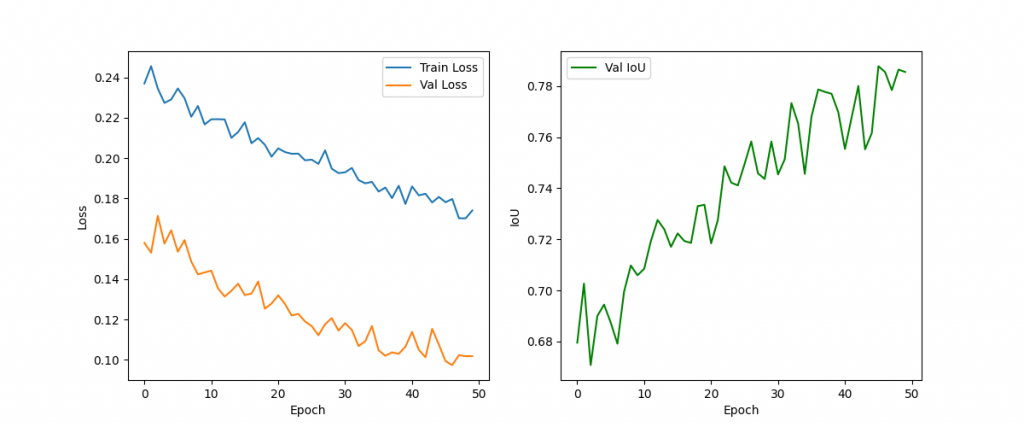
Visualize Results
This visualize_results function is a utility to check how well the trained U²-Net predicts segmentation masks on random samples from the dataset. It loads the saved model checkpoint, picks a random image-mask pair from the dataset, runs inference, and thresholds the predicted mask at 0.5. It then calculates the Intersection over Union (IoU) score between the predicted and ground-truth masks as a quantitative measure. Finally, it creates a visualization with three side-by-side plots: the original input image, the ground truth mask, and the predicted mask annotated with the IoU. This gives both a qualitative and quantitative sense of the model’s performance on unseen data.
def visualize_results(model_path, dataset, device):
    # Load the trained model
    model = U2NETP(in_ch=3, out_ch=1).to(device)
    checkpoint = torch.load(model_path, map_location=device)
    model.load_state_dict(checkpoint['model_state_dict'])
    model.eval()
    print("Model loaded successfully")

    # Select a random sample from the dataset
    idx = random.randint(0, len(dataset)-1)
    image, true_mask = dataset[idx]
    image = image.unsqueeze(0).to(device)  # Add batch dimension

    # Run inference
    with torch.no_grad():
        pred_mask, _, _, _, _, _, _ = model(image)

    # Convert to numpy arrays
    image_np = image.squeeze().cpu().numpy().transpose(1, 2, 0)
    true_mask_np = true_mask.squeeze().cpu().numpy()
    pred_mask_np = pred_mask.squeeze().cpu().numpy()

    # Threshold the prediction
    pred_mask_np = (pred_mask_np > 0.5).astype(np.float32)

    # Calculate metrics
    intersection = np.logical_and(true_mask_np, pred_mask_np)
    union = np.logical_or(true_mask_np, pred_mask_np)
    iou = np.sum(intersection) / np.sum(union)

    # Create figure
    plt.figure(figsize=(15, 5))

    # Original Image
    plt.subplot(1, 3, 1)
    plt.imshow(image_np)
    plt.title('Original Image')
    plt.axis('off')

    # True Mask
    plt.subplot(1, 3, 2)
    plt.imshow(true_mask_np, cmap='gray')
    plt.title('Ground Truth Mask')
    plt.axis('off')

    # Predicted Mask
    plt.subplot(1, 3, 3)
    plt.imshow(pred_mask_np, cmap='gray')
    plt.title(f'Predicted Mask (IoU: {iou:.4f})')
    plt.axis('off')

    plt.tight_layout()
    plt.show()

# Path to your saved model
model_path = '/U2-Net/Model/best_u2net_small.pth'

# Visualize results on test dataset
visualize_results(model_path, test_dataset, device)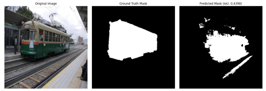
Removing Background
Your visualize_and_extract function is designed to let you upload any custom image, run it through the trained U²-Net model, and extract the salient foreground object i.e. removes the background.
def load_model(model_path, device):
    model = U2NETP(in_ch=3, out_ch=1).to(device)
    checkpoint = torch.load(model_path, map_location=device)
    model.load_state_dict(checkpoint['model_state_dict'])
    model.eval()
    print("Model loaded successfully")
    return model

def visualize_and_extract(model_path, device):
    # Upload file
    uploaded = files.upload()
    image_path = list(uploaded.keys())[0]
    print(f"Uploaded file: {image_path}")

    # Load the trained model
    model = load_model(model_path, device)

    # Define preprocessing
    transform = transforms.Compose([
        transforms.Resize((320, 320)),   # match training size
        transforms.ToTensor(),
    ])

    # Load and preprocess uploaded image
    image = Image.open(image_path).convert("RGB")
    input_tensor = transform(image).unsqueeze(0).to(device)

    # Run inference
    with torch.no_grad():
        pred_mask, _, _, _, _, _, _ = model(input_tensor)

    # Convert to numpy
    image_resized = image.resize((320, 320))
    image_np = np.array(image_resized)
    pred_mask_np = pred_mask.squeeze().cpu().numpy()
    pred_mask_np = (pred_mask_np > 0.5).astype(np.uint8)  # binary mask (0,1)

    # Extract salient feature
    salient_np = image_np * pred_mask_np[:, :, np.newaxis]  # apply mask

    # Plot results
    plt.figure(figsize=(15, 5))

    # Original image
    plt.subplot(1, 3, 1)
    plt.imshow(image_np)
    plt.title("Uploaded Image")
    plt.axis("off")

    # Predicted mask
    plt.subplot(1, 3, 2)
    plt.imshow(pred_mask_np, cmap="gray")
    plt.title("Predicted Mask")
    plt.axis("off")

    # Extracted salient feature
    plt.subplot(1, 3, 3)
    plt.imshow(salient_np)
    plt.title("Extracted Foreground")
    plt.axis("off")

    plt.tight_layout()
    plt.show()

    # Optionally save extracted image
    salient_img = Image.fromarray(salient_np.astype(np.uint8))
    salient_img.save("salient_feature.png")
    print("Foreground saved as salient_feature.png")


# Path to your saved model
model_path = '/U2-Net/Model/best_u2net_small.pth'
visualize_and_extract(model_path, device)